AAanalysis Cheat Sheet

v1.1 Cheat Sheet

Sequence → physicochemical scales → interpretable features → explainable ML → biological mechanism

pip install aaanalysis · aaanalysis.readthedocs.io

AAanalysis is a Python framework for interpretable, sequence-based protein prediction. It turns sequences into physicochemical features (CPP), trains explainable models, and traces every prediction back to a residue × property × group comparison — robust for small datasets. v1.1 extends the core feature engine beyond physicochemical scales to PLM embeddings and protein structure.

Install · Import · Loadcore + [pro]

# Python >= 3.11
pip install aaanalysis         # core
pip install 'aaanalysis[pro]'  # SHAP, FIMO, Bio

import numpy as np
import matplotlib.pyplot as plt
import aaanalysis as aa
df_seq = aa.load_dataset(name='DOM_GSEC')   # γ-secretase
labels = df_seq['label'].to_list()
df_scales = aa.load_scales()

The Golden Workflowcanonical pipeline

1LOADload_dataset · load_scales→df_seq · df_scales

2PARTSSequenceFeature.get_df_parts→df_parts

3FEATURESPart × Split × Scale · CPP.run→df_feat

4MODELTreeModel.fit · dPULearn.fit→feat_importance · labels_

5EXPLAINCPPPlot.feature_map · ShapModel→figure · feat_impact

Prediction Task Levelstask → setup

Residue AA_*positional

unit: sliding window (aa_window_size)

ref: non-site windows / shuffled background

Domain DOM_*both

unit: part-set jmd_n · tmd · jmd_c (from tmd_start / tmd_stop)

ref: labelled A vs B groups

Protein SEQ_*compositional

unit: whole chain (composition)

ref: labelled groups / composition-matched background

Output types: classification · regression · ranking · explanation

Groups:1: positives0: negatives0: reliable negatives2: unlabeled

Label 0 is a curated negative in labelled data, or a dPULearn-inferred reliable negative drawn from the unlabeled (2) pool.

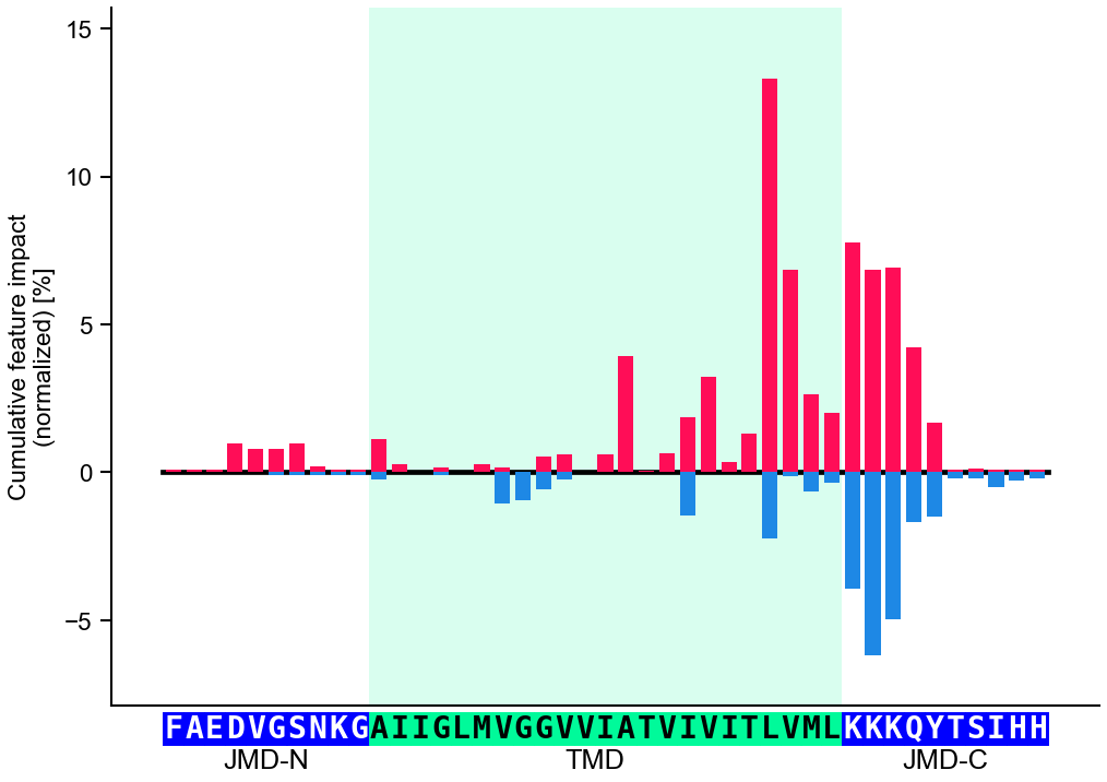
Sequence Anatomythe TMD model

TMD	Target Middle Domain — the central segment of interest (e.g. transmembrane domain); variable length.
JMD	Juxta Middle Domain — the fixed-width flanks adjoining the TMD (jmd_n on the N-side, jmd_c on the C-side).

JMD-N

TMD

JMD-C

0tmd_starttmd_stoplen(seq)

JMD widths set globally: aa.options['jmd_n_len'] · ['jmd_c_len'].

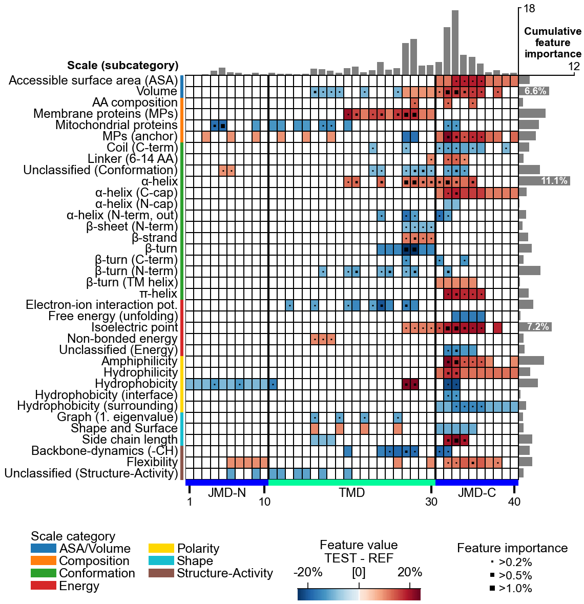
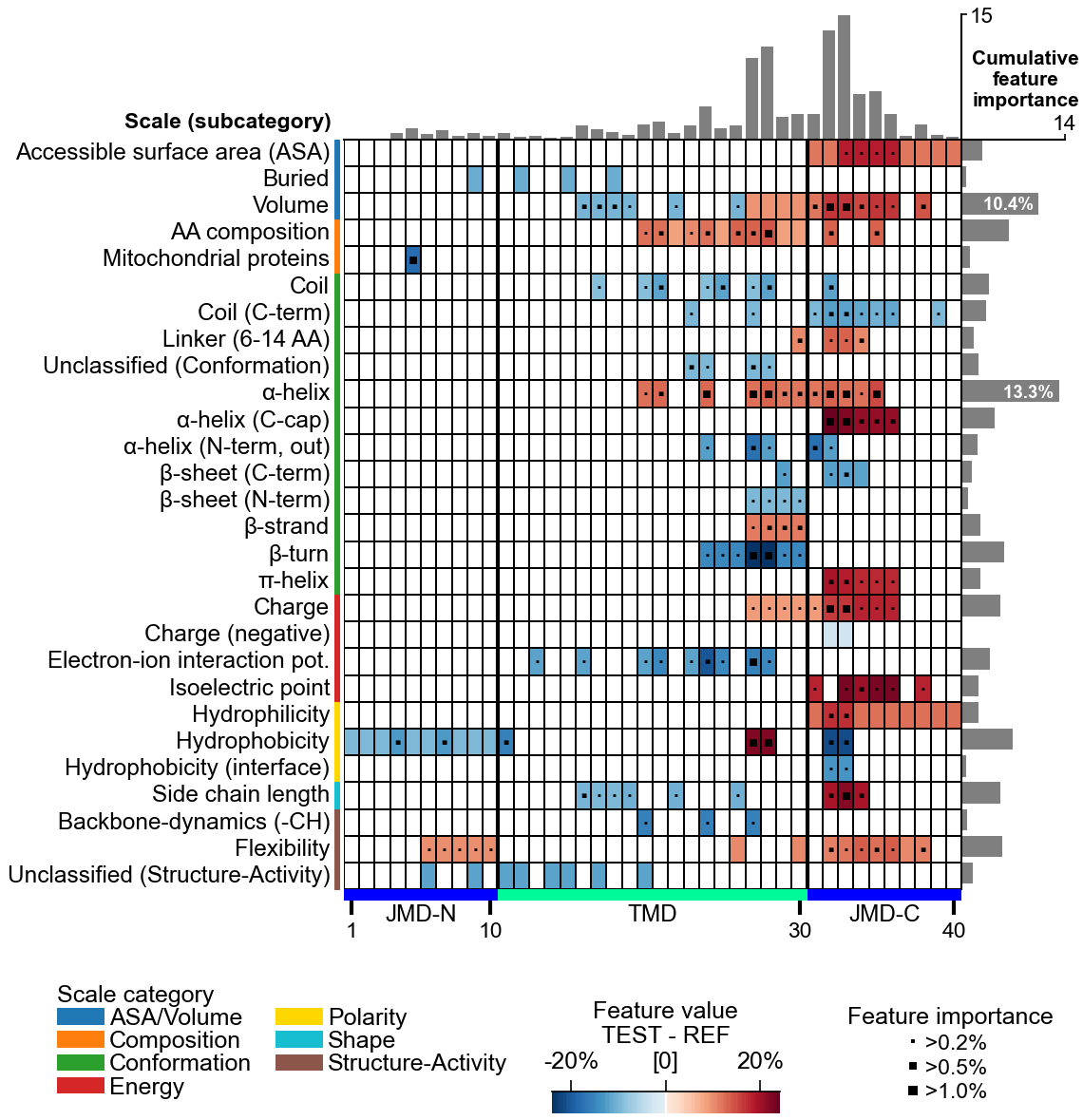
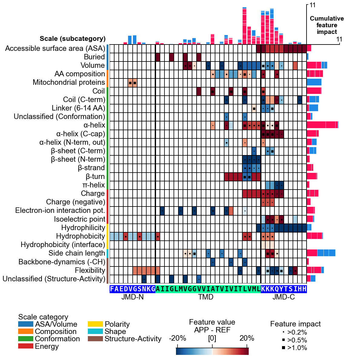
CPP Feature ConceptPart × Split × Scale

PART where on the sequence

tmd · jmd_n · jmd_c · tmd_jmd · jmd_n_tmd_n · tmd_c_jmd_c

SPLIT how to read the part

Segment — contiguous · Pattern — sparse pairs · PeriodicPattern — i, i+3/4

SCALE which physicochemical property

AAontology (~600 scales) · hydrophobicity · charge · helix propensity

TMDA I I G L M V G G V V I

Segment(1,4)■ ■ ■ · · · · · · · · ·

Pattern(N,1,4,8)■ · · ■ · · · ■ · · · ·

PeriodicPattern■ · · ■ · · ■ · · ■ · ·

Splitting maps parts (of various length) to fixed relative positions.

Simplified from Breimann25 (Suppl. Fig. 1C ↗)

TMD × Segment × hydrophobicity → membrane insertion

JMD × Pattern × net charge → electrostatic recognition

TMD × PeriodicPattern × helix → α-helical interface

CPP Strategiesvia split_kws

Compositional ≈ sequence/protein-level

one whole-part average (composition-like, position-agnostic)

split_kws = sf.get_split_kws(
    split_types="Segment",
    n_split_max=1)
cpp = aa.CPP(df_parts=df_parts, split_kws=split_kws)

Positional ≈ residue-/region-level

sub-segments and/or patterns resolved to positions

split_kws = sf.get_split_kws(
    split_types=["Segment", "Pattern", "PeriodicPattern"],
    n_split_max=5,
    steps_pattern=[3, 4],
    steps_periodicpattern=[3, 4])
cpp = aa.CPP(df_parts=df_parts, split_kws=split_kws)

Domain level uses both. → CPP strategies: see the CPP tutorial (docs).

See details in Breimann25 · Suppl. Fig. 1 ↗

Which Module Should I Use?intent → module

Explore sequence patterns / compositionAAlogo

Sample reference windows (if negatives are missing)AAWindowSampler

Reduce redundant amino acid scalesAAclust

Discover discriminative physicochemical featuresCPP

Train with positives + unlabeled datadPULearn

Train an interpretable classifierTreeModel

Explain a prediction (per feature / sample)ShapModel pro

Data & Preparationdatasets · scales · FASTA

Load benchmark sequencesload_dataset(name) → df_seq

Load AAontology scalesload_scales() → df_scales

Load precomputed featuresload_features(name) → df_feat

Read / write FASTAread_fasta(file) → df_seq

Cluster redundant homologsfilter_seq(df_seq) → df_clust pro

Sequence Analysislogos · windows · motifs

Position-specific logoAAlogo().get_df_logo(df_parts) → df_logo

Sample reference windowsAAWindowSampler().sample_*(df_seq)

Pairwise sequence similaritycomp_seq_sim(df_seq) pro

Scan motifs (FIMO / MEME)scan_motif(df_seq, pwm) → df_hits pro

Feature Engineeringparts · CPP · scales

SequenceFeature → sfsf = aa.SequenceFeature()

· split sequence into partssf.get_df_parts(df_seq) → df_parts

· assemble feature matrix Xsf.feature_matrix(df_feat, df_parts) → X

Discover discriminative featuresCPP(df_parts).run(labels) → df_feat ★

Sweep CPP configs (grid)CPPGrid().run(...) · .eval() → ranked configs

Simplify → interpretable scalesCPP.simplify(df_feat, labels) → df_feat

Reduce redundant scalesAAclust().fit(X) [Wrapper]

Drop correlated featuresNumericalFeature().filter_correlation(X)

Feature Preprocessingone-hot · PLM · structure · PTM

Encode sequences (one-hot / int)SequencePreprocessor().encode_*(seqs) → X

PLM embeddings v1.1EmbeddingPreprocessor().encode(...) → dict_num

Structure / DSSP / PAE v1.1StructurePreprocessor().encode_dssp(...) → dict_num pro

PTM / site annotations v1.1AnnotationPreprocessor().encode(...) → dict_num pro

Combine sources v1.1combine_dict_nums([...]) → dict_num

Numerical CPP v1.1CPP(df_parts).run_num(dict_num_parts, labels) → df_feat

Modeling & ExplainabilityPU · classify · SHAP

Train with positives + unlabeled datadPULearn().fit(X, labels) [Wrapper]

Train + RFE + MC importanceTreeModel().fit(X, labels) [Wrapper]

Per-feature / sample SHAP impactShapModel().fit(X, labels) pro

Metrics & Plottingmetrics · plots

Adjusted AUC (class imbalance)comp_auc_adjusted(X, labels)

BIC score · KL divergencecomp_bic_score(X, labels) · comp_kld

Per-protein / detection (v1.1)comp_per_protein_ap · comp_detection_metrics

Plot style, fonts & standalone legendplot_settings(font_scale) · plot_legend(ax)

Protein Design (to be extended)mutations · design

In-silico point mutations v1.1AAMut · AAMutPlot

Sequence-design libraries v1.1SeqMut · SeqMutPlot

AAlogo — see the datadataset at a glance

import numpy as np, matplotlib.pyplot as plt, aaanalysis as aa
df_seq = aa.load_dataset(name='DOM_GSEC')   # γ-secretase
labels = list(df_seq['label']); df_scales = aa.load_scales()
sf = aa.SequenceFeature()
df_parts = sf.get_df_parts(df_seq=df_seq,
    list_parts=['tmd', 'jmd_n', 'jmd_c'])
aa.plot_settings(font_scale=0.7)
# aal_kws builds df_logo + bits bar for you
aa.AAlogoPlot().single_logo(
    aal_kws=dict(df_parts=df_parts, labels=labels,
        label_test=1, tmd_len=20),
    name_data='Test set: substrates')
plt.tight_layout(); plt.show()

AAlogoPlot.single_logo · per-position enrichment

CPP — featuretop feature · test vs ref

# default parts + a redundancy-reduced set of 100 scales
df_parts = sf.get_df_parts(df_seq=df_seq)
df_scales = aa.AAclust().select_scales(
    df_scales=df_scales, n_clusters=100)
cpp = aa.CPP(df_parts=df_parts, df_scales=df_scales)
df_feat = cpp.run(labels=labels, n_filter=100)
X = sf.feature_matrix(df_feat['feature'], df_parts)
tm = aa.TreeModel(); tm.fit(X, labels=labels)
df_feat = tm.add_feat_importance(df_feat=df_feat, sort=True)
cpp_plot = aa.CPPPlot(); aa.plot_settings()
# distribution of the top feature (feat_rank=1 of the sorted df_feat)
cpp_plot.feature(feature=df_feat, feat_rank=1, df_seq=df_seq,
    labels=labels, name_test='substrates', name_ref='non-subs.')
plt.tight_layout(); plt.show()

▼ figure below · left

CPP — rankingtop features · effect + importance

# same df_feat — rank the top discriminative features
aa.plot_settings(font_scale=0.6)
cpp_plot.ranking(df_feat=df_feat, n_top=15, rank=True,
    name_test='substrates', name_ref='non-subs.')
plt.tight_layout(); plt.show()

▼ figure below · right

CPP — ranking — CPPPlot.ranking · top-15 features

CPP — feature mapgroup level · importance

# global Part × Split × Scale map — all AAontology scales
cpp_plot = aa.CPPPlot(); aa.plot_settings(font_scale=0.65)
cpp_plot.feature_map(df_feat=df_feat)
# CPP.simplify → fewer, interpretable correlated scales
df_feat = cpp.simplify(df_feat=df_feat, labels=labels)
cpp_plot.feature_map(df_feat=df_feat)
plt.tight_layout(); plt.show()

ShapModel — explain a predictionsample level · [pro]

# per-sample SHAP — APP's soft label (0.6), keyed by entry
sm = aa.ShapModel()
sm.fit(X, labels=labels, df_seq=df_seq,
       fuzzy_labels={'P05067': 0.6})
df_feat = sm.add_feat_impact(df_feat=df_feat, df_seq=df_seq,
                             samples='P05067', names='APP')
args_seq = sf.get_args_seq(df_seq=df_seq, sample='P05067')
ka = dict(col_imp='feat_impact_APP', shap_plot=True, **args_seq)
cpp_plot.profile(df_feat=df_feat, **ka)
# vmin/vmax=±21% → same colour scale as the global feature map (comparable)
cpp_plot.feature_map(df_feat=df_feat, name_test='APP',
                     vmin=-21, vmax=21, **ka)
plt.tight_layout(); plt.show()

See details in Breimann25 · Suppl. Fig. 10 ↗

AAclust — clustersscale reduction · clustering

aac = aa.AAclust()
# pick a redundancy-reduced set of scales
aac.select_scales(df_scales, n_clusters=10)
aac.medoid_names_   # 10 reduced scales (labels_ also set)

aac_plot = aa.AAclustPlot()
aac_plot.centers(df_scales=df_scales, labels=aac.labels_)
plt.tight_layout(); plt.show()

# AAclust also reduces redundant proteins (not just scales)
df_seq = aac.select_proteins(df_seq=df_seq, X=X)

▼ figure below · left

dPULearn — PCAreliable negatives · PU learning

# DOM_GSEC ships 1/0 — treat 0 as the unlabeled pool (label_unl=0)
dpul = aa.dPULearn()
dpul.fit(X=X, labels=labels, label_unl=0, n_neg=31)   # n_neg: reliable negatives to mine
df_pu = dpul.df_pu_   # out: 1 pos · 0 rel-neg · 2 unl

dpul_plot = aa.dPULearnPlot()
dpul_plot.pca(df_pu=df_pu, labels=dpul.labels_)
plt.tight_layout(); plt.show()

▼ figure below · right

AAclust — clusters — AAclustPlot.centers · cluster scale profiles

dPULearn — PCA — dPULearnPlot.pca · reliable negatives

See details in Breimann25 · Suppl. Fig. 3 ↗

AAWindowSamplerbuild reference windows

# Reference windows around sites when you lack negatives:
aaws = aa.AAWindowSampler()
# SAME proteins · window 9 (odd) -> PTM / single-residue site
df_same = aaws.sample_same_protein(df_seq, n=100, window_size=9)
# DIFFERENT proteins · window 10 (even) -> cleavage bond
df_diff = aaws.sample_different_protein(df_seq, n=100, window_size=10)
# SYNTHETIC — AA-frequency priors (null background)
df_syn = aaws.sample_synthetic(df_seq, n=100, generator='global_freq')

Decision Guidepick your setup

What are you predicting?

per residue / site → AA_* · odd/even window · parts = window

per domain / region → DOM_* · TMD model · parts = jmd_n·tmd·jmd_c

whole protein → SEQ_* · composition · whole chain

What labels do you have?

labeled 0 / 1 → CPP → ML model

positives + unlabeled (1 / 2) → CPP → dPULearn → ML model

no negatives at all → AAWindowSampler → CPP → ML model

What is your learning task?

classify → CPP → classifier (sklearn)

regress → get_labels_quantile / tiered → CPP → regression model

multi-class → get_labels_ovr / ovo → CPP → classifiers

cluster → AAclust

Which explainability do you need?

group level → CPP → TreeModel → CPPPlot → feature importance

per protein → CPP → ShapModel pro → CPPPlot → feature impact ↑↓

Gotchasthings that bite

Labels: 1/0 = supervised (pos/neg). dPULearn takes 1/0 (label_unl=0) or 1/2; n_neg = reliable negatives to mine; output 1 · 0 (rel-neg) · 2 (unl).
load_dataset(name, n=N) returns 2N rows (N per class) — count classes via df_seq['label'].
Compositional vs positional is not a flag — it emerges from split_kws.
Reproducibility: layered seeds — seed= ▸ random_state= ▸ options['random_state'] ▸ default.
DOM_* parts need tmd_start/tmd_stop in df_seq; [pro] features need pip install 'aaanalysis[pro]'.

Design Principlesthe AAanalysis way

Explicit over implicit — DataFrames everywhere
Wrappers (.fit / .predict / .eval) set trailing *_ attributes after fit
Biological interpretability is first-class
Small-data robust and reproducible (layered seeds)

Key Data Objectsshapes & columns

df_seq	entry · sequence · label · tmd_start · tmd_stop
df_parts	one column per part: tmd · jmd_n · jmd_c · …
df_feat	feature · category · subcategory · scale_name · abs_auc · mean_dif · p_val · positions
X	feature matrix (samples × features) from sf.feature_matrix
dict_num	{entry: ndarray (L×D)} — numerical per-residue values

Class · abbr ↔ Plot Classmirrored API

class	abbr	plot class	kind
SequencePreprocessor	sp	—
EmbeddingPreprocessor	ep	—
StructurePreprocessor pro	stp	—
AnnotationPreprocessor pro	ap	—
AAlogo	aal	AAlogoPlot
AAWindowSampler	aaws	—
SequenceFeature	sf	—
NumericalFeature	nf	—
AAclust	aac	AAclustPlot	Wrapper
CPP	cpp	CPPPlot
dPULearn	dpul	dPULearnPlot	Wrapper
TreeModel	tm	—	Wrapper
ShapModel pro	sm	—	Wrapper
AAMut	aamut	AAMutPlot
SeqMut	seqmut	SeqMutPlot

aa.optionssystem-level settings

aa.options['random_state'] = 42
aa.options['verbose'] = True
aa.options['n_jobs'] = -1            # all cores (None = auto)
aa.options['allow_multiprocessing'] = True

# TMD model — JMD flank widths
aa.options['jmd_n_len'] = 10
aa.options['jmd_c_len'] = 10

# plot labels & system-level scales
aa.options['name_tmd'] = 'P5-P5′'   # e.g. cleavage site
aa.options['df_scales'] = my_scales

How to Citeif you use AAanalysis

[Breimann24a]AAclust

Breimann & Frishman (2024a), AAclust: k-optimized clustering for selecting redundancy-reduced sets of amino acid scales

Bioinformatics Advances ↗

[Breimann24b]AAontology

Breimann et al. (2024b), AAontology: An ontology of amino acid scales for interpretable machine learning

Journal of Molecular Biology ↗

[Breimann25]CPP & dPULearn

Breimann & Kamp et al. (2025), Charting γ-secretase substrates by explainable AI

Nature Communications ↗

Glossarycanonical vocabulary · CONTEXT.md

Feature (CPP) — (Part × Split × Scale) — the atomic, residue-grounded, interpretable unit of CPP.

Part — Named segment used as feature input: tmd, jmd_n, jmd_c, tmd_jmd, jmd_n_tmd_n, tmd_c_jmd_c.

TMD (Target Middle Domain) — The central variable-length sequence segment of interest, made comparable across samples by splitting. Called “transmembrane domain” in Breimann25, but generalized here to any target segment.

JMD (Juxta Middle Domain) — The fixed-length flanking regions adjacent to the TMD: jmd_n (N-terminal side) and jmd_c (C-terminal side); called “juxtamembrane domain” in Breimann25.

Split — How a scale is read across a part: Segment (contiguous), Pattern (sparse), PeriodicPattern (i, i+3/4).

Scale — AA (amino acid) → ℝ mapping. AAontology ships ~600 curated scales in two-level categories.

AAontology — Two-level scale taxonomy; CPP uses its categories to organize and rank features.

CPP — Comparative Physicochemical Profiling — discovers ranked Part × Split × Scale features.

Test vs reference group — The A-vs-B contrast CPP profiles: a feature's mean_dif is test − reference (name_test / name_ref in CPPPlot).

Compositional vs positional — How split_kws resolves locality: a whole-part average (compositional) vs sub-region/position-resolved (positional).

Numerical CPP (pseudo-scale) v1.1 — CPP generalizes from AA→scale lookup to any per-residue tensor — PLM (protein language model) · structure (PDB file) · functional annotations (e.g. PTMs) — each a pseudo-scale via CPP.run_num.

Feature importance vs impact — Two explainability axes: importance = unsigned, group-level (TreeModel); impact = signed, per-sample (ShapModel, shap_plot).

Reducing features — Four distinct ops: redundancy reduction (AAclust scales) · feature pruning · selection (RFE, recursive feature elimination) · simplification (CPP.simplify → interpretable scales).

PU learning (Positive-Unlabeled learning) — Training from labeled positives and unlabeled data only (no curated negatives); dPULearn infers reliable negatives from the unlabeled pool.

PU labels — dPULearn input: 1 = positive, 2 = unlabeled. Output: 1 / 0 (reliable-negative) / 2.

Wrapper class — sklearn-style class — .fit / .predict / .eval, sets trailing *_ attributes after fit.

Plot class — *Plot mirror of an analytical class — same arguments, visualization only.