Quick start with AAanalysis

This is a short introduction to AAanalysis, a Python framework for sequence-based protein prediction, centered around the Comparative Physical Profiling (CPP) algorithm for interpretable feature engineering.

First, import some third-party packages and aanalysis:

import seaborn as sns
import matplotlib.pyplot as plt
import pandas as pd
import numpy as np

import aaanalysis as aa
aa.options["verbose"] = False
aa.options["random_state"] = 42

Data Loading

We can load a dataset of amino acid scales using the aa.load_scales() function. Dataset of protein sequences for a binary classification task, such as our γ-secretase substrates (n=63) and non-substrates (n=63) dataset ([Breimann25a]), can be retrieved via the aa.load_dataest() function:

# Load example dataset and scales
df_seq = aa.load_dataset(name="DOM_GSEC")
labels = list(df_seq["label"])
df_scales = aa.load_scales()

Feature Engineering

To start feature engineering, we can utilize the AAclust model for selecting a redundancy-reduced set of amino acid scales:

# Obtain redundancy-reduced set of 100 scales
aac = aa.AAclust()
X = np.array(df_scales).T
scales = aac.fit(X, names=list(df_scales), n_clusters=100).medoid_names_
df_scales = df_scales[scales]

We can now use the CPP algorithm, which aims at identifying a set of features that are most discriminant between two sets of sequences. It´s core idea is the CPP feature concept, defined as a combination of Parts, Splits, and Scales. Parts and Splits can be obtained using SequenceFeature.

We first create a set of baseline features:

sf = aa.SequenceFeature()

# Obtain Parts and Splits
df_parts = sf.get_df_parts(df_seq=df_seq, list_parts=["tmd"])
split_kws = sf.get_split_kws(n_split_max=1, split_types=["Segment"])

Running CPP via CPP.run() creates all Part-Split-Scale combinations and filters them down to a user-defined maximum of non-redundant features (100 by default). As baseline, we use CPP without filtering (max_cor=1) to compute the average values for the 100 selected scales over the entire TMD sequences:

# Create 100 baseline features (Scale values averaged over TMD)
cpp = aa.CPP(df_scales=df_scales, df_parts=df_parts, split_kws=split_kws)
df_feat_baseline = cpp.run(labels=labels, max_cor=1)
aa.display_df(df=df_feat_baseline, n_rows=8)

	feature	category	subcategory	scale_name	scale_description	abs_auc	abs_mean_dif	mean_dif	std_test	std_ref	p_val_mann_whitney	p_val_fdr_bh	positions
1	TMD-Segment(1,1)-WOLR790101	Polarity	Hydrophobicity (surrounding)	Hydration potential	Hydrophobicity ...n et al., 1979)	0.257000	0.037000	0.037000	0.028000	0.042000	0.000001	0.000064	11,12,13,14,15,...,26,27,28,29,30
2	TMD-Segment(1,1)-FUKS010106	Composition	Membrane proteins (MPs)	Proteins of mesophiles (INT)	Interior compos...ishikawa, 2001)	0.240000	0.068000	0.068000	0.065000	0.082000	0.000003	0.000160	11,12,13,14,15,...,26,27,28,29,30
3	TMD-Segment(1,1)-BEGF750103	Conformation	β-turn	β-turn	Conformational ...in-Dirkx, 1975)	0.237000	0.064000	-0.064000	0.067000	0.087000	0.000004	0.000147	11,12,13,14,15,...,26,27,28,29,30
4	TMD-Segment(1,1)-FASG760105	Polarity	Unclassified (Polarity)	pK-C	pK-C (Fasman, 1976)	0.234000	0.044000	0.044000	0.038000	0.057000	0.000006	0.000142	11,12,13,14,15,...,26,27,28,29,30
5	TMD-Segment(1,1)-YUTK870104	Energy	Free energy (unfolding)	Free energy (unfolding)	Activation Gibb...i et al., 1987)	0.234000	0.011000	0.011000	0.010000	0.020000	0.000006	0.000121	11,12,13,14,15,...,26,27,28,29,30
6	TMD-Segment(1,1)-LINS030116	ASA/Volume	Accessible surface area (ASA)	ASA (folded β-strand)	Total median ac...s et al., 2003)	0.230000	0.028000	-0.028000	0.021000	0.039000	0.000008	0.000137	11,12,13,14,15,...,26,27,28,29,30
7	TMD-Segment(1,1)-ANDN920101	Structure-Activity	Backbone-dynamics (-CH)	α-CH chemical s...kbone-dynamics)	alpha-CH chemic...n et al., 1992)	0.229000	0.068000	-0.068000	0.073000	0.081000	0.000009	0.000102	11,12,13,14,15,...,26,27,28,29,30
8	TMD-Segment(1,1)-ROBB760109	Conformation	β-turn (N-term)	β-turn (1st residue)	Information mea...n-Suzuki, 1976)	0.229000	0.039000	-0.039000	0.041000	0.047000	0.000009	0.000115	11,12,13,14,15,...,26,27,28,29,30

By default, CPP creates around 100,000 Part-Slit combinations:

# CPP creates around 100,000 features and filters them down to 100
df_parts = sf.get_df_parts(df_seq=df_seq)
cpp = aa.CPP(df_scales=df_scales, df_parts=df_parts)
df_feat = cpp.run(labels=labels)
aa.display_df(df=df_feat, n_rows=8)

	feature	category	subcategory	scale_name	scale_description	abs_auc	abs_mean_dif	mean_dif	std_test	std_ref	p_val_mann_whitney	p_val_fdr_bh	positions
1	TMD_C_JMD_C-Seg...2,3)-QIAN880106	Conformation	α-helix	α-helix (middle)	Weights for alp...ejnowski, 1988)	0.387000	0.118000	0.118000	0.068000	0.080000	0.000000	0.000000	27,28,29,30,31,32,33
2	TMD_C_JMD_C-Pat...,12)-ROBB760109	Conformation	β-turn (N-term)	β-turn (1st residue)	Information mea...n-Suzuki, 1976)	0.363000	0.119000	-0.119000	0.065000	0.085000	0.000000	0.000000	21,25,28,32
3	TMD_C_JMD_C-Seg...6,9)-ZIMJ680104	Energy	Isoelectric point	Isoelectric point	Isoelectric poi...n et al., 1968)	0.352000	0.268000	0.268000	0.174000	0.173000	0.000000	0.000000	32,33
4	TMD_C_JMD_C-Seg...4,9)-ROBB760113	Conformation	β-turn	β-turn	Information mea...n-Suzuki, 1976)	0.349000	0.337000	-0.337000	0.177000	0.254000	0.000000	0.000000	27,28
5	TMD_C_JMD_C-Seg...4,5)-ZIMJ680104	Energy	Isoelectric point	Isoelectric point	Isoelectric poi...n et al., 1968)	0.336000	0.205000	0.205000	0.134000	0.157000	0.000000	0.000000	33,34,35,36
6	TMD_C_JMD_C-Pat...,15)-QIAN880106	Conformation	α-helix	α-helix (middle)	Weights for alp...ejnowski, 1988)	0.336000	0.152000	0.152000	0.102000	0.132000	0.000000	0.000000	28,32,35
7	TMD_C_JMD_C-Seg...6,9)-LINS030101	ASA/Volume	Volume	Accessible surface area (ASA)	Total accessibl...s et al., 2003)	0.328000	0.235000	0.235000	0.156000	0.187000	0.000000	0.000000	32,33
8	TMD_C_JMD_C-Seg...2,3)-ZIMJ680104	Energy	Isoelectric point	Isoelectric point	Isoelectric poi...n et al., 1968)	0.326000	0.108000	0.108000	0.077000	0.085000	0.000000	0.000000	27,28,29,30,31,32,33

Machine Learning (Protein Prediction)

A feature matrix for a given set of CPP features can be created using the SequenceFeature.feature_matrix() method. The feature matrix will be used to train a Random Forest Classifier model:

from sklearn.ensemble import RandomForestClassifier
from sklearn.model_selection import cross_val_score

# Create feature matrix and perform prediction for baseline features
X = sf.feature_matrix(df_parts=df_parts, features=df_feat_baseline["feature"])
rf = RandomForestClassifier()
cv_base = cross_val_score(rf, X, labels, scoring="accuracy", cv=5)
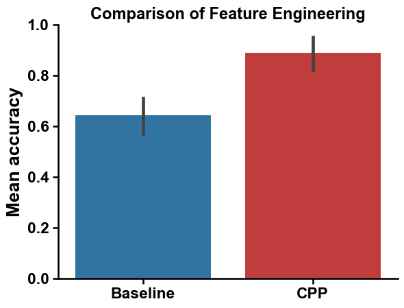
print(f"Mean accuracy of {round(np.mean(cv_base), 2)}")

Mean accuracy of 0.64

We create now the feature matrix for the features obtained with CPP default settings:

# Create feature matrix and perform prediction for default CPP features
X = sf.feature_matrix(df_parts=df_parts, features=df_feat["feature"])
rf = RandomForestClassifier()
cv = cross_val_score(rf, X, labels, scoring="accuracy", cv=5)
print(f"Mean accuracy of {round(np.mean(cv), 2)}")

Mean accuracy of 0.89

We can compare the baseline and default CPP feature set using a bar chart:

# Comparison of baseline and default CPP feature sets
aa.plot_settings()
sns.barplot(pd.DataFrame({"Baseline": cv_base, "CPP": cv}), palette=["tab:blue", "tab:red"])
plt.ylabel("Mean accuracy", size=aa.plot_gcfs()+1)
plt.ylim(0, 1)
plt.title("Comparison of Feature Engineering", size=aa.plot_gcfs()-1)
sns.despine()
plt.show()

CPP Analysis (group level)

AAanalysis offers various plotting functions for interpreting the CPP features at group and sample level by CPPPlot. We first need to include the group-level feature importance using the TreeModel and its TreeModel.add_feat_importance() method:

# Include group level feature importance
tm = aa.TreeModel()
tm.fit(X, labels=labels)
df_feat = tm.add_feat_importance(df_feat=df_feat)

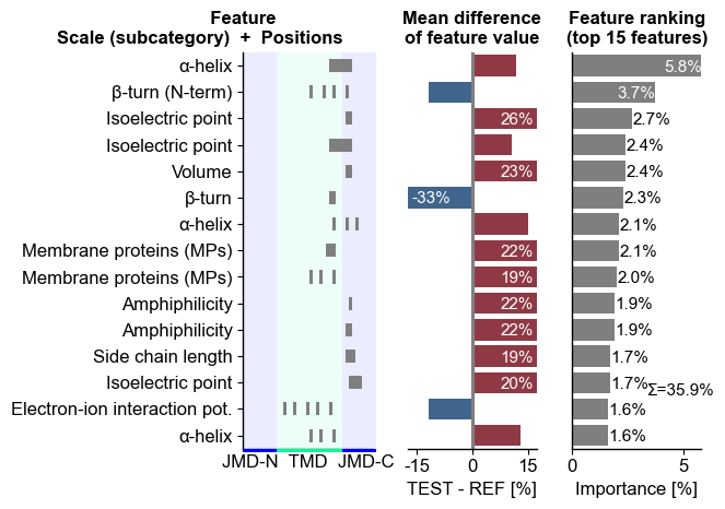
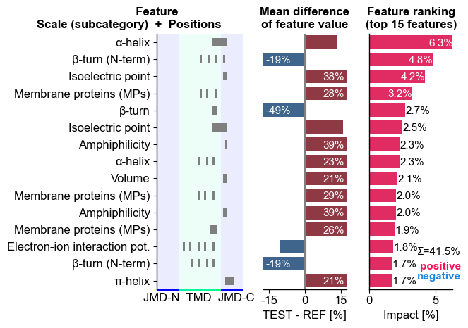
The top15 features can be displayed using the CPPPlot.ranking() method:

# Plot CPP ranking
cpp_plot = aa.CPPPlot()
aa.plot_settings(short_ticks=True, weight_bold=False)
cpp_plot.ranking(df_feat=df_feat)
plt.tight_layout()
plt.show()

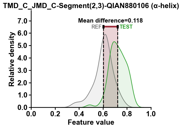
The distributions of features values for the highest-ranked feature can be displayed using the CPPPlot.feature() method:

top_feature = df_feat["feature"][0]
top_subcategory = df_feat["subcategory"][0]
aa.plot_settings()
cpp_plot.feature(feature=top_feature , df_seq=df_seq, labels=labels)
plt.title(f"{top_feature} ({top_subcategory})")
plt.tight_layout()
plt.show()

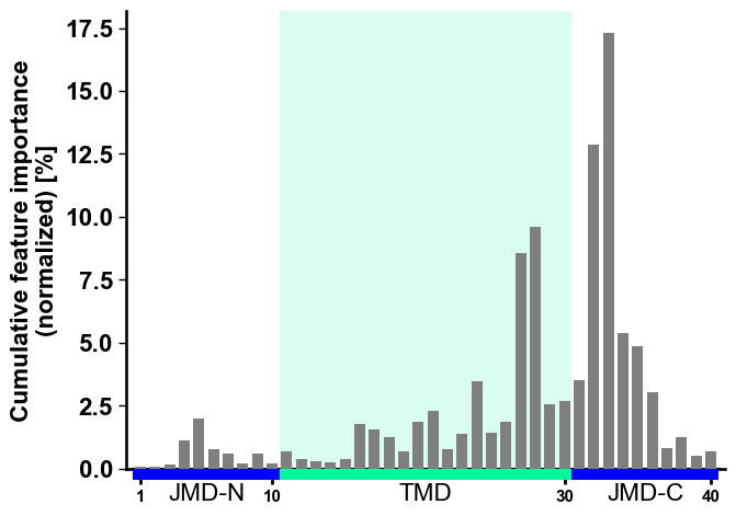
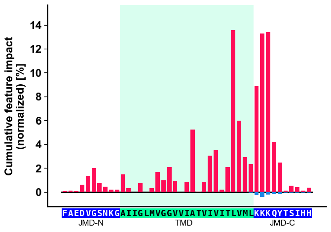
The cumulative feature importance per residue position can be visualized by the CPPPlot.profile() method:

# Plot CPP profile
aa.plot_settings(font_scale=0.9)
cpp_plot.profile(df_feat=df_feat)
plt.tight_layout()
plt.show()

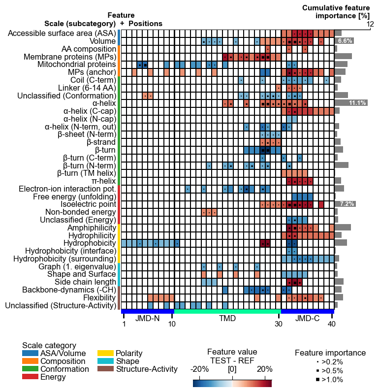
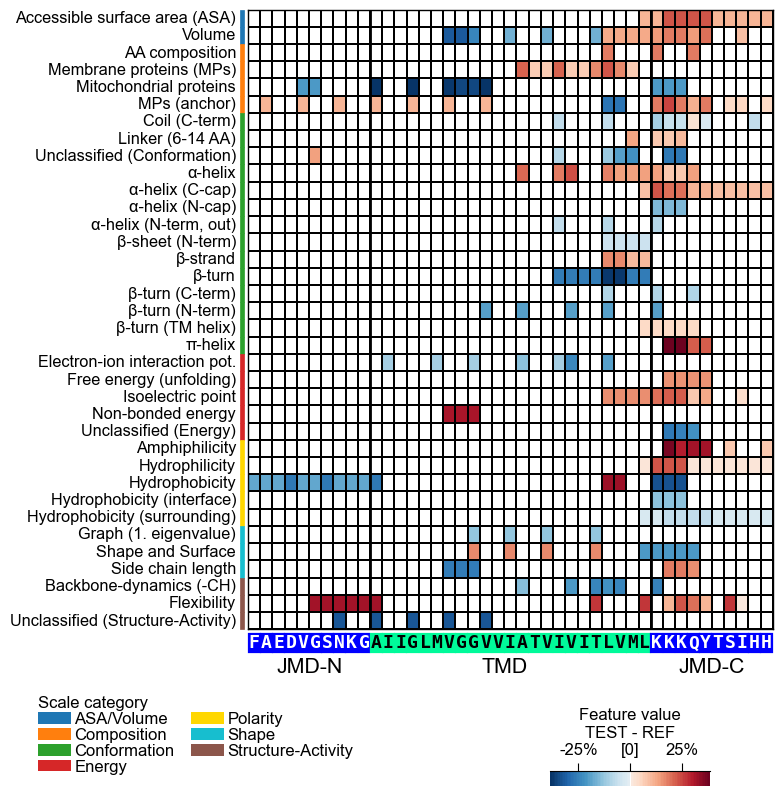
To uncover the common physicochemical signature discriminating the test from the reference protein set, use the CPPPlot.feature_map() method showing the feature value differences per scale subcategory at single-residue resolution:

# Plot CPP feature map (original version: without importance bars on top)
cpp_plot = aa.CPPPlot()
aa.plot_settings(font_scale=0.65, weight_bold=False)
cpp_plot.feature_map(df_feat=df_feat, add_imp_bar_top=False)
plt.show()

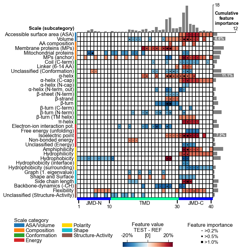
# Plot CPP feature map (v1.0.2+: with importance bars on top)
cpp_plot = aa.CPPPlot()
aa.plot_settings(font_scale=0.65, weight_bold=False)
cpp_plot.feature_map(df_feat=df_feat)
plt.show()

CPP-SHAP Analysis (sample level)

We can analyse the impact of features on the prediction score for individual sequence using the ShapExplainer model, which combines CPP with the explainable AI framework SHAP.

# Obtain sample-specific feature impact
sm = aa.ShapModel()
sm.fit(X, labels=labels)
df_feat = sm.add_feat_impact(df_feat=df_feat)
df_feat = sm.add_sample_mean_dif(X, labels=labels, df_feat=df_feat)

We can now show the feature ranking for a selected protein (‘Protein0’) using the CPPPlot.ranking() method, plotting SHAP analysis results by setting shap_plot=True:

# CPP-SHAP ranking plot
aa.plot_settings(short_ticks=True, weight_bold=False)
cpp_plot.ranking(df_feat=df_feat, shap_plot=True, col_dif="mean_dif_Protein0", col_imp="feat_impact_Protein0")
plt.tight_layout()
plt.show()

To visualize the CPP-SHAP profile and heatmap, we need to obtain the sequence parts of the respective protein:

# Get sequences parts for APP
_df_parts = sf.get_df_parts(df_seq=df_seq, list_parts=["tmd", "jmd_c", "jmd_n"])
_args_seq = _df_parts.loc["P05067"].to_dict()
args_seq = {key + "_seq": _args_seq[key] for key in _args_seq}

Show the specific CPP-SHAP Profile for the first Protein using the CPPPlot.profile() method with setting shap_plot=True:

# CPP-SHAP profile
aa.plot_settings(font_scale=0.9)
cpp_plot.profile(df_feat=df_feat, shap_plot=True, col_imp="feat_impact_Protein0", **args_seq)
plt.tight_layout()
plt.show()

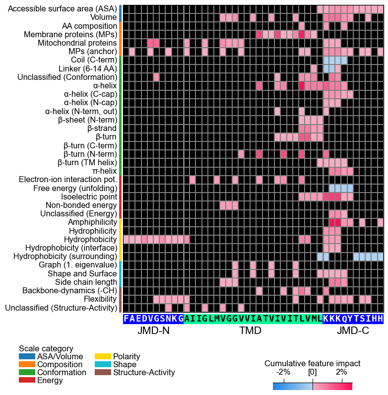
With the CPPPlot.heatmap() we can visualize the sample-specific feature value difference and the feature impact per scale subcategory and residue position:

# CPP heatmap (sample level)
aa.plot_settings(font_scale=0.65, weight_bold=False)
cpp_plot.heatmap(df_feat=df_feat, shap_plot=True, col_val="mean_dif_Protein0", **args_seq)
plt.show()

# CPP-SHAP heatmap (sample level)
cpp_plot.heatmap(df_feat=df_feat, shap_plot=True, col_val="feat_impact_Protein0", **args_seq)
plt.show()

See our Feature Engineering API for a comprehensive documentation on the CPP, CPPPlot, AAclust, and SequenceFeature classes.