Slow start with AAanalysis

Dive into the powerful capabilities of AAanalysis—a Python framework for sequence-based (i.e., alignment-free) and interpretable protein prediction. In this tutorial, we’ll focus on extracting physicochemical features from protein sequences using the Comparative Physical Profiling (CPP) algorithm and how these features can be harnessed for binary classification tasks.

What You Will Learn

1. Data Loadings: Load protein sequences and selections of amino acid scales.

2. Feature Engineering: Extract essential features using the AAclust and CPP models.

3. Machine Learning: Make predictions using the RandomForest model.

4. Explainable AI: Interpret predictions at the group and individual levels by combining CPP with SHAP.

import seaborn as sns
import matplotlib.pyplot as plt
import pandas as pd
import numpy as np

import aaanalysis as aa
aa.options["verbose"] = False
aa.options["random_state"] = 42

1. Data Loading

With AAanalysis, you have access to numerous benchmark datasets for sequence-based protein prediction, mainly for binary classification tasks. You can retrieve these datasets with the aa.load_dataset() function. Amino acid scales, predominantly from AAindex, along with their two-level hierarchical classification (AAontology, [Breimann24b]), are available with the aa.load_scales() function. See AAontology Usage Principels for further details.

We first load the complete scales dataset and our primary example dataset from [Breimann25a]_ of γ-secretase substrates (n=63) and non-substrates (n=63):

# Load example dataset and scales
df_seq = aa.load_dataset(name="DOM_GSEC")
labels = list(df_seq["label"])
df_scales = aa.load_scales()

2. Feature Engineering

The centerpiece of AAanalysis is the CPP model, which is supported by AAclust, a clustering wrapper framework for the pre-selection of amino acid scales, which was introduced in [Breimann24a].

AAclust

Since redundancy is an essential problem for machine learning tasks, the AAclust object provides a lightweight wrapper for sklearn clustering algorithms such as Agglomerative clustering. AAclust clusters a set of scales and selects for each cluster the most representative scale (i.e., the scale closes to the cluster center). More details can be found in AAclust Usage Principels.

We will use AAclust to obtain a set of 100 scales, as defined by the n_clusters parameters:

# Obtain redundancy-reduced set of 100 scales
aac = aa.AAclust()
X = np.array(df_scales).T
scales = aac.fit(X, names=list(df_scales), n_clusters=100).medoid_names_
df_scales = df_scales[scales]

Comparative Physicochemical Profiling (CPP)

CPP is a sequence-based algorithm for interpretable feature engineering, introduced in [Breimann25a]. It aims at identifying a set of features most discriminant between two sets of sequences: the test set and the reference set. The core idea of CPP is its feature concepts, which integrates:

• Parts: Are combination of a target middle domain (TMD) and N- and C-terminal adjacent regions (JMD-N and JMD-C, respectively), obtained sf.get_df_parts.

• Splits: These Parts can be split into various continuous segments or discontinuous patterns, specified sf.get_split_kws().

• Scales: Sets of amino acid scales (or other numerical scales).

See CPP Usage Principles for more conceptual background.

We use the supporting SequenceFeature class to obtain Parts and Splits. These together with the Scales are used by CPP as input to identify the set of characteristic features to discriminate between both datasets, such as γ-secretase substrates and non-substrates:

sf = aa.SequenceFeature()

# Obtain Parts and Splits
df_parts = sf.get_df_parts(df_seq=df_seq, list_parts=["tmd"])
split_kws = sf.get_split_kws(n_split_max=1, split_types=["Segment"])

Performing the CPP algorithm using the CPP.run() method creates all Part-Split-Split combinations and filters them down to a user-defined maximum of non-redundant features (100 by default). As baseline, we use CPP without filtering (max_cor=1) to compute the average values for the 100 selected scales over the entire TMD sequences:

# Create 100 baseline features (Scale values averaged over TMD)
cpp = aa.CPP(df_scales=df_scales, df_parts=df_parts, split_kws=split_kws)
df_feat_baseline = cpp.run(labels=labels, max_cor=1)
aa.display_df(df=df_feat_baseline, n_rows=8)

	feature	category	subcategory	scale_name	scale_description	abs_auc	abs_mean_dif	mean_dif	std_test	std_ref	p_val_mann_whitney	p_val_fdr_bh	positions
1	TMD-Segment(1,1)-WOLR790101	Polarity	Hydrophobicity (surrounding)	Hydration potential	Hydrophobicity ...n et al., 1979)	0.257000	0.037000	0.037000	0.028000	0.042000	0.000001	0.000064	11,12,13,14,15,...,26,27,28,29,30
2	TMD-Segment(1,1)-FUKS010106	Composition	Membrane proteins (MPs)	Proteins of mesophiles (INT)	Interior compos...ishikawa, 2001)	0.240000	0.068000	0.068000	0.065000	0.082000	0.000003	0.000160	11,12,13,14,15,...,26,27,28,29,30
3	TMD-Segment(1,1)-BEGF750103	Conformation	β-turn	β-turn	Conformational ...in-Dirkx, 1975)	0.237000	0.064000	-0.064000	0.067000	0.087000	0.000004	0.000147	11,12,13,14,15,...,26,27,28,29,30
4	TMD-Segment(1,1)-FASG760105	Polarity	Unclassified (Polarity)	pK-C	pK-C (Fasman, 1976)	0.234000	0.044000	0.044000	0.038000	0.057000	0.000006	0.000142	11,12,13,14,15,...,26,27,28,29,30
5	TMD-Segment(1,1)-YUTK870104	Energy	Free energy (unfolding)	Free energy (unfolding)	Activation Gibb...i et al., 1987)	0.234000	0.011000	0.011000	0.010000	0.020000	0.000006	0.000121	11,12,13,14,15,...,26,27,28,29,30
6	TMD-Segment(1,1)-LINS030116	ASA/Volume	Accessible surface area (ASA)	ASA (folded β-strand)	Total median ac...s et al., 2003)	0.230000	0.028000	-0.028000	0.021000	0.039000	0.000008	0.000137	11,12,13,14,15,...,26,27,28,29,30
7	TMD-Segment(1,1)-ANDN920101	Structure-Activity	Backbone-dynamics (-CH)	α-CH chemical s...kbone-dynamics)	alpha-CH chemic...n et al., 1992)	0.229000	0.068000	-0.068000	0.073000	0.081000	0.000009	0.000102	11,12,13,14,15,...,26,27,28,29,30
8	TMD-Segment(1,1)-ROBB760109	Conformation	β-turn (N-term)	β-turn (1st residue)	Information mea...n-Suzuki, 1976)	0.229000	0.039000	-0.039000	0.041000	0.047000	0.000009	0.000115	11,12,13,14,15,...,26,27,28,29,30

CPP uses 330 Splits and 3 Parts by default, yielding around 100,000 features when using 100 Scales. Creating and filtering all these Part-Split-Scale combinations will take a little time (about 25 seconds for this example on an i7-10510U (4 cores, 8 threads) with multiprocessing), but it significantly improves prediction performance:

# CPP creates around 100,000 features and filters them down to 100
df_parts = sf.get_df_parts(df_seq=df_seq)
cpp = aa.CPP(df_scales=df_scales, df_parts=df_parts)
df_feat = cpp.run(labels=labels)
aa.display_df(df=df_feat, n_rows=8)

	feature	category	subcategory	scale_name	scale_description	abs_auc	abs_mean_dif	mean_dif	std_test	std_ref	p_val_mann_whitney	p_val_fdr_bh	positions
1	TMD_C_JMD_C-Seg...2,3)-QIAN880106	Conformation	α-helix	α-helix (middle)	Weights for alp...ejnowski, 1988)	0.387000	0.118000	0.118000	0.068000	0.080000	0.000000	0.000000	27,28,29,30,31,32,33
2	TMD_C_JMD_C-Pat...,12)-ROBB760109	Conformation	β-turn (N-term)	β-turn (1st residue)	Information mea...n-Suzuki, 1976)	0.363000	0.119000	-0.119000	0.065000	0.085000	0.000000	0.000000	21,25,28,32
3	TMD_C_JMD_C-Seg...6,9)-ZIMJ680104	Energy	Isoelectric point	Isoelectric point	Isoelectric poi...n et al., 1968)	0.352000	0.268000	0.268000	0.174000	0.173000	0.000000	0.000000	32,33
4	TMD_C_JMD_C-Seg...4,9)-ROBB760113	Conformation	β-turn	β-turn	Information mea...n-Suzuki, 1976)	0.349000	0.337000	-0.337000	0.177000	0.254000	0.000000	0.000000	27,28
5	TMD_C_JMD_C-Seg...4,5)-ZIMJ680104	Energy	Isoelectric point	Isoelectric point	Isoelectric poi...n et al., 1968)	0.336000	0.205000	0.205000	0.134000	0.157000	0.000000	0.000000	33,34,35,36
6	TMD_C_JMD_C-Pat...,15)-QIAN880106	Conformation	α-helix	α-helix (middle)	Weights for alp...ejnowski, 1988)	0.336000	0.152000	0.152000	0.102000	0.132000	0.000000	0.000000	28,32,35
7	TMD_C_JMD_C-Seg...6,9)-LINS030101	ASA/Volume	Volume	Accessible surface area (ASA)	Total accessibl...s et al., 2003)	0.328000	0.235000	0.235000	0.156000	0.187000	0.000000	0.000000	32,33
8	TMD_C_JMD_C-Seg...2,3)-ZIMJ680104	Energy	Isoelectric point	Isoelectric point	Isoelectric poi...n et al., 1968)	0.326000	0.108000	0.108000	0.077000	0.085000	0.000000	0.000000	27,28,29,30,31,32,33

3. Machine Learning (Protein Prediction)

A feature matrix for a given set of CPP features can be created using the sf.feat_matrix() method. The feature matrix will be used to train a Random Forest Classifier model:

from sklearn.ensemble import RandomForestClassifier
from sklearn.model_selection import cross_val_score

# Create feature matrix and perform prediction for baseline features
X = sf.feature_matrix(df_parts=df_parts, features=df_feat_baseline["feature"])
rf = RandomForestClassifier()
cv_base = cross_val_score(rf, X, labels, scoring="accuracy", cv=5)
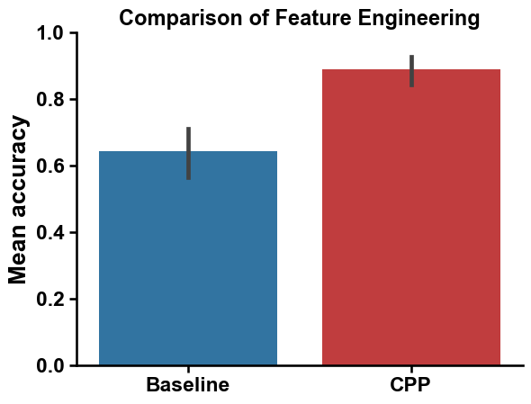
print(f"Mean accuracy of {round(np.mean(cv_base), 2)}")

Mean accuracy of 0.64

We create now the feature matrix for the features obtained with CPP default settings:

# Create feature matrix and perform prediction for default CPP features
X = sf.feature_matrix(df_parts=df_parts, features=df_feat["feature"])
rf = RandomForestClassifier()
cv = cross_val_score(rf, X, labels, scoring="accuracy", cv=5)
print(f"Mean accuracy of {round(np.mean(cv), 2)}")

Mean accuracy of 0.89

We can compare the baseline and default CPP feature set using a bar chart:

# Comparison of baseline and default CPP feature sets
aa.plot_settings()
sns.barplot(pd.DataFrame({"Baseline": cv_base, "CPP": cv}), palette=["tab:blue", "tab:red"])
plt.ylabel("Mean accuracy", size=aa.plot_gcfs()+1)
plt.ylim(0, 1)
plt.title("Comparison of Feature Engineering", size=aa.plot_gcfs()-1)
sns.despine()
plt.show()

CPP Analysis

AAanalysis offers a range of plotting functions through the CPPPlot class for interpreting the features identified by CPP. For a binary classification tasks, the CPP features and their machine learning-based importance can be visualized at two different levels:

• Group level: Highlights the differences and feature importance between two groups, aiding in their discrimination.

• Sample level: Shows differences between an individual sample and a reference group, along with the importance of specific features.

CPP Analysis (group level)

To obtain the group level feature importance, we developed the TreeModel class. It is a wrapper for tree-based models from scikit-learn or similar libraries XGBoost or CatBoost. The TreeModel obtains a Monte Carlo estimate of the importance of each feature by training different models over multiple iterations and averaging their results. These estimates can be included into the feature DataFrame (df_feat) using the TreeModel.add_feat_importance() method:

# Include group level feature importance
tm = aa.TreeModel()
tm.fit(X, labels=labels)
df_feat = tm.add_feat_importance(df_feat=df_feat)

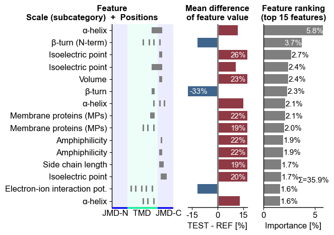
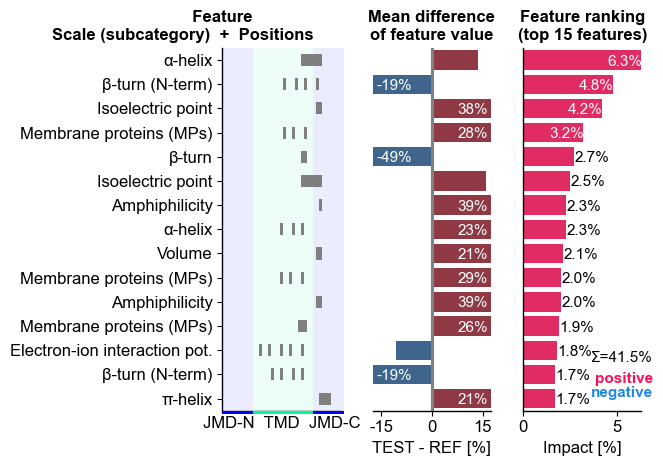
The top15 features can be displayed using the CPPPlot.ranking() method. The features are shown (left) as a combination of the scale subcategory and their position derived from the Part-Split combination. The difference of feature values between the test and reference set of protein (here γ-secretase substrates and non-substrates) is shown in the middle. The right subplots displays the feature importance used for ranking:

# Plot CPP ranking
cpp_plot = aa.CPPPlot()
aa.plot_settings(short_ticks=True, weight_bold=False)
cpp_plot.ranking(df_feat=df_feat)
plt.tight_layout()
plt.show()

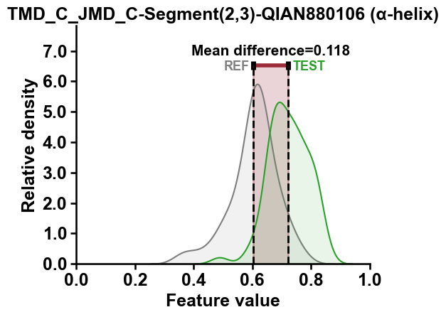
The distributions of features values for the highest-ranked feature can be displayed using the CPPPlot.feature() method, which shows the distribution for the test (‘Test’) and reference (‘REF’) dataset along with the difference of their mean values (‘Mean difference’):

top_feature = df_feat["feature"][0]
top_subcategory = df_feat["subcategory"][0]
aa.plot_settings()
cpp_plot.feature(feature=top_feature , df_seq=df_seq, labels=labels)
plt.title(f"{top_feature} ({top_subcategory})")
plt.tight_layout()
plt.show()

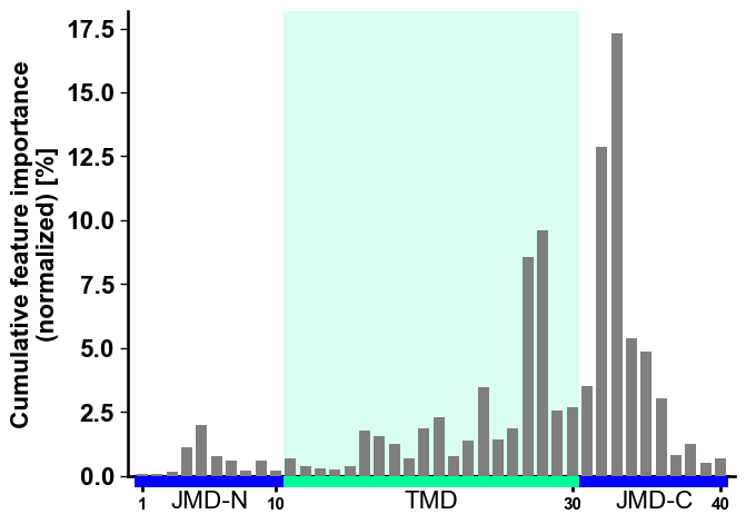
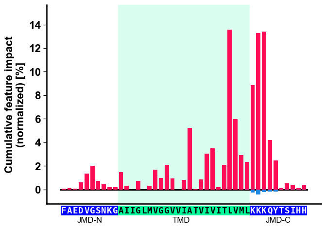
To visualize the importance of all features at single-residue resolution, the cumulative feature importance per residue position can be shown using the CPPPlot.profile() method. As this method presents group level results, it allows for the adjustment of the lengths of different Parts:

# Plot CPP profile
aa.plot_settings(font_scale=0.9)
cpp_plot.profile(df_feat=df_feat)
plt.tight_layout()
plt.show()

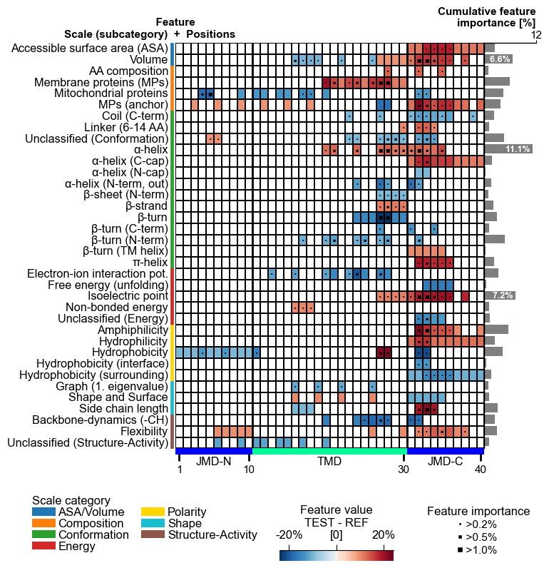
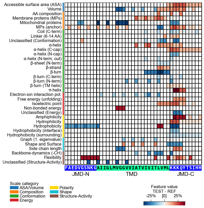
The centerpiece of the AAanalysis package is the feature map, which shows the common physicochemical signature for discriminating the test from the reference protein set. It is created by the `CPPPlot.feature_map()`` method showing the feature value differences per scale subcategory at single-residue resolution:

# Plot CPP feature map (original version: without importance bars on top)
cpp_plot = aa.CPPPlot()
aa.plot_settings(font_scale=0.65, weight_bold=False)
cpp_plot.feature_map(df_feat=df_feat, add_imp_bar_top=False)
plt.show()

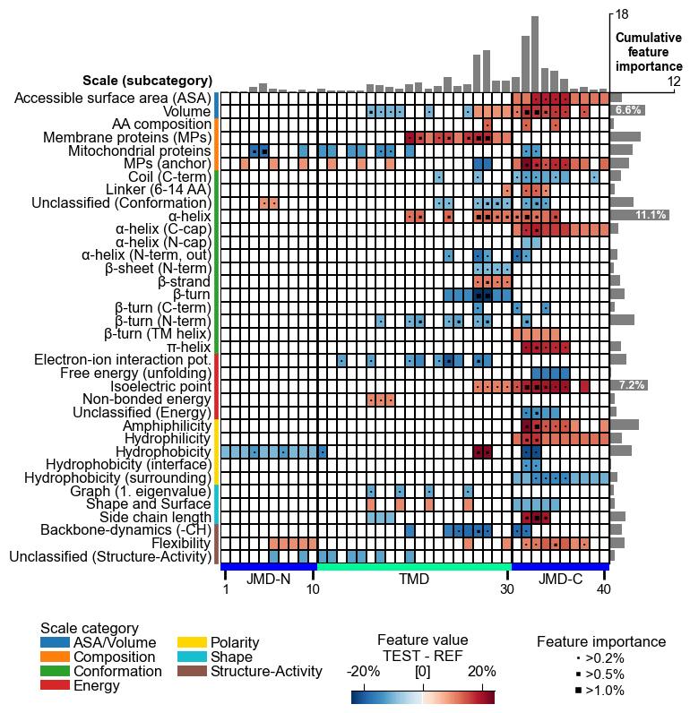
# Plot CPP feature map (v1.0.2+: with importance bars on top)
cpp_plot = aa.CPPPlot()
aa.plot_settings(font_scale=0.65, weight_bold=False)
cpp_plot.feature_map(df_feat=df_feat)
plt.show()

4. Explainable AI

CPP-SHAP Analysis (sample level)

We can analyse the impact of features on the prediction score for individual sequence using the ShapModel model, which combines CPP with the explainable AI framework SHAP.

# Obtain sample-specific feature impact
sm = aa.ShapModel()
sm.fit(X, labels=labels)
df_feat = sm.add_feat_impact(df_feat=df_feat)
df_feat = sm.add_sample_mean_dif(X, labels=labels, df_feat=df_feat)

To explain the feature impact with single-residue resolution, AAanalysis offers the following four types of visualizations: CPP-SHAP ranking plot, CPP-SHAP profile, CPP heatmap, CPP-SHAP heatmap. An overview is provided under Explainable AI Usage Principles

We can now show the feature ranking for a selected protein (‘Protein0’) using the CPPPlot.ranking() method, plotting SHAP analysis results by setting shap_plot=True:

# CPP-SHAP ranking plot
aa.plot_settings(short_ticks=True, weight_bold=False)
cpp_plot.ranking(df_feat=df_feat, shap_plot=True, col_dif="mean_dif_Protein0", col_imp="feat_impact_Protein0")
plt.tight_layout()
plt.show()

To visualize the CPP-SHAP profile and heatmap, we need to obtain the sequence parts of the respective protein:

# Get sequences parts for APP
_df_parts = sf.get_df_parts(df_seq=df_seq, list_parts=["tmd", "jmd_c", "jmd_n"])
_args_seq = _df_parts.loc["P05067"].to_dict()
args_seq = {key + "_seq": _args_seq[key] for key in _args_seq}

Show the specific CPP-SHAP Profile for the first Protein using the CPPPlot.profile() method with setting shap_plot=True:

# CPP-SHAP profile
aa.plot_settings(font_scale=0.9)
cpp_plot.profile(df_feat=df_feat, shap_plot=True, col_imp="feat_impact_Protein0", **args_seq)
plt.tight_layout()
plt.show()

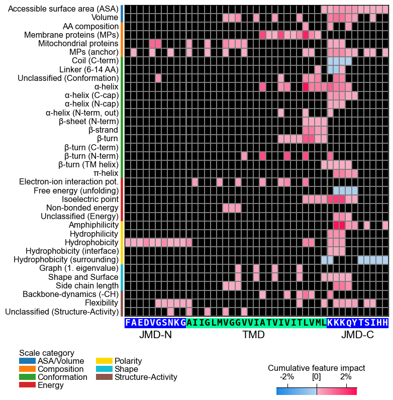
With the CPPPlot.heatmap() method we can visualize the sample-specific feature value difference and the feature impact per scale subcategory and residue position. Set shap_plot=True and provide the respective column with the mean difference and the feature impact:

# CPP heatmap (sample level)
aa.plot_settings(font_scale=0.65, weight_bold=False)
cpp_plot.heatmap(df_feat=df_feat, shap_plot=True, col_val="mean_dif_Protein0", **args_seq)
plt.show()

# CPP-SHAP heatmap (sample level)
cpp_plot.heatmap(df_feat=df_feat, shap_plot=True, col_val="feat_impact_Protein0", **args_seq)
plt.show()

See our Feature Engineering API for a comprehensive documentation on the CPP, CPPPlot, AAclust, and SequenceFeature classes.