Charting γ-secretase substrates by explainable AI

Showcase a published study with AAanalysis. Where a tutorial teaches one tool and a protocol teaches one workflow, a use case walks through a real study end-to-end from bundled data only (no downloads) — showing that a published result drops out of the standard AAanalysis pipeline, and serving as a template you adapt to your own data.

This use case showcases the study:

Breimann and Kamp et al. (2025), Charting γ-secretase substrates by explainable AI, Nature Communications 16, 5428.

Biological motivation. γ-secretase is an intramembrane-cleaving protease that cuts the transmembrane domain of single-span membrane proteins, releasing fragments that drive signalling — and it is central to Alzheimer’s disease (it generates the amyloid-β peptide from the amyloid precursor protein, APP) and to cancer (it activates Notch receptors). Yet out of hundreds of single-span membrane proteins, γ-secretase cleaves only a subset, and no consensus sequence motif marks which ones. Worse, the data is weakly labelled: a few dozen expert-curated substrates, only a handful of confirmed non-substrates, and hundreds of proteins of unknown status. The study asks what physicochemically defines a substrate, and how to predict substrates despite this.

The AAanalysis pipeline. Comparative Physicochemical Profiling (CPP) builds an interpretable, position-resolved signature of the substrates over a redundancy-reduced set of amino-acid scales (curated with AAclust); deterministic Positive-Unlabelled learning (dPULearn) mines reliable negatives from the unlabelled pool to balance the data; a tree model predicts substrate status; and SHAP explains individual predictions at single-residue resolution.

What this showcases (key steps, simplified). Sequence logos of the three protein groups · an AAclust redundancy-reduced scale set · the CPP signature and feature map with importances · dPULearn reliable-negative mining · a prediction benchmark (feature engineering × data expansion) and feature-number optimization · single-residue SHAP explanations for individual substrates.

Simplifications (so it runs in seconds). The study works over the full human N-out proteome across ten model types with leave-one-out CV and three transmembrane annotations. Here we use the bundled balanced DOM_GSEC set (63 substrates + 63 reliable non-substrates) and the unlabelled DOM_GSEC_PU set (63 substrates + 631 others) with their single embedded TMHMM annotation, one tree ensemble, and 5-fold cross-validation. The biology and the headline numbers come through; scaling up is the Protocols (P1, P4, P7-P10).

import numpy as np
import pandas as pd
import matplotlib.pyplot as plt
import seaborn as sns
from sklearn.cluster import AgglomerativeClustering
from sklearn.svm import SVC
from sklearn.ensemble import RandomForestClassifier
from sklearn.linear_model import LogisticRegression
from sklearn.calibration import CalibratedClassifierCV
from xgboost import XGBClassifier
from sklearn.model_selection import cross_val_predict, LeaveOneOut
from sklearn.metrics import balanced_accuracy_score

import aaanalysis as aa

aa.options["verbose"] = False
aa.options["random_state"] = 42
JMD_LEN = 10
sf = aa.SequenceFeature()

# Canonical group names + colours (defined ONCE, used in every plot; from the AAanalysis palette).
dict_color = aa.plot_get_cdict(name="DICT_COLOR")
NAME_SUB = "Substrate"                          # positives: experimentally confirmed substrates
NAME_NONSUB = "Non-substrate"                   # both negative subgroups combined
NAME_NONSUB_KNOWN = "Non-substrate (known)"     # experimentally-known negatives (14)
NAME_NONSUB_DPU = "Non-substrate (dPULearn)"    # reliable negatives mined by dPULearn (49)
NAME_OTHERS = "Others"                          # the unlabelled proteins (candidate substratome)
C_SUB = dict_color["SAMPLES_POS"]               # substrate / positive (green)
C_NONSUB_KNOWN = dict_color["SAMPLES_NEG"]      # non-substrate, known (magenta)
C_NONSUB_DPU = dict_color["SAMPLES_REL_NEG"]    # non-substrate, dPULearn (gold)
C_OTHERS = dict_color["SAMPLES_UNL"]            # Others / unlabelled (gray)
C_NONSUB = "#a34e2f"                            # both negative subgroups combined (dark red)
# Prediction-confidence bands (study SHAP gradient) for score-based colouring:
C_HC_SUB, C_HC_NON = dict_color["SHAP_POS"], dict_color["SHAP_NEG"]   # SHAP palette endpoints (red / blue)
C_LC_SUB, C_LC_NON = dict_color["SHAP_POS_LC"], dict_color["SHAP_NEG_LC"]
DICT_GROUP_COLOR = {NAME_SUB: C_SUB, NAME_NONSUB_KNOWN: C_NONSUB_KNOWN,
                    NAME_NONSUB_DPU: C_NONSUB_DPU, NAME_OTHERS: C_OTHERS}

# Shared benchmark evaluator (as in the study): a linear SVM under leave-one-out CV, scored by
# balanced accuracy.
def balanced_acc(X, y):
    y = np.asarray(y)
    y_pred = cross_val_predict(SVC(kernel="linear"), X, y, cv=LeaveOneOut(), n_jobs=-1)
    return balanced_accuracy_score(y, y_pred) * 100

1. Load the data

Two bundled domain-level (DOM_) datasets, one row per protein with the transmembrane geometry and the pre-cut jmd_n / tmd / jmd_c parts:

• ``DOM_GSEC`` — the curated balanced set: 63 substrates (label=1) + 63 reliable non-substrates (label=0).

• ``DOM_GSEC_PU`` — the positive-unlabelled set: the same 63 substrates + 631 unlabelled proteins of unknown status (label=2, the “others”).

TMD annotation. The jmd_n / tmd / jmd_c split depends on where each protein’s transmembrane domain (TMD) sits — predicted from the sequence by a TMD-annotation model (which residues span the membrane, hence the boundaries defining the flanking JMD-N / JMD-C). The study combined three annotations (UniProt, Phobius, TMHMM) for robustness; here we use only TMHMM for convenience, and the headline numbers still come through.

# 14 experimentally-known non-substrates retrieved from literature at the start of the study.
list_non_sub = ["P50895", "Q9Y624", "Q14802", "P05556", "P49257", "Q86UE4", "P16234",
                "Q969W9", "P53801", "Q8IUW5", "Q9NPR2", "P01135", "Q96JJ7", "O43914"]
_df_gsec = aa.load_dataset(name="DOM_GSEC")
_df_gsec_pu = aa.load_dataset(name="DOM_GSEC_PU")

# Split the raw data into the three biological groups of interest.
df_sub = _df_gsec[_df_gsec["label"] == 1]                     # curated substrates
df_non_sub = _df_gsec[_df_gsec["entry"].isin(list_non_sub)]   # curated non-substrates
df_unl = _df_gsec_pu[_df_gsec_pu["label"] == 2]               # unlabelled "others" (unknown status)

# Two working sets: CPP features come from substrates vs unlabelled (the raw signal); the ML
# benchmark is substrates vs the 14 experimentally-known non-substrates, exactly as in the study.
df_sub_nonsub = pd.concat([df_sub, df_non_sub]).reset_index(drop=True)  # 63 + 14 (benchmark)
df_sub_unl = pd.concat([df_sub, df_unl]).reset_index(drop=True)          # 63 + 631 (feature generation)
labels_sub_nonsub = (df_sub_nonsub["label"] == 1).astype(int).to_numpy() # 1 substrate, 0 non-substrate
labels_sub_unl = (df_sub_unl["label"] == 1).astype(int).to_numpy()       # 1 substrate, 0 unlabelled

print(f"Substrates: {len(df_sub)} | non-substrates: {len(df_non_sub)} | unlabelled: {len(df_unl)}")
print(f"Feature set (substrate vs unlabelled): {len(df_sub_unl)} | benchmark (substrate vs non-substrate): {len(df_sub_nonsub)}")
aa.display_df(df=df_sub_nonsub, n_rows=10, show_shape=True)

Substrates: 63 | non-substrates: 14 | unlabelled: 631
Feature set (substrate vs unlabelled): 694 | benchmark (substrate vs non-substrate): 77
DataFrame shape: (77, 9)

	entry	gene	sequence	label	tmd_start	tmd_stop	jmd_n	tmd	jmd_c
1	P05067	APP	MLPGLALLLLAAWTA...GYENPTYKFFEQMQN	1	701	723	FAEDVGSNKG	AIIGLMVGGVVIATVIVITLVML	KKKQYTSIHH
2	P14925	Pam	MAGRARSGLLLLLLG...EEEYSAPLPKPAPSS	1	868	890	KLSTEPGSGV	SVVLITTLLVIPVLVLLAIVMFI	RWKKSRAFGD
3	P70180	Npr3	MRSLLLFTFSACVLL...RELREDSIRSHFSVA	1	477	499	PCKSSGGLEE	SAVTGIVVGALLGAGLLMAFYFF	RKKYRITIER
4	Q03157	Aplp1	MGPTSPAARGQGRRW...HGYENPTYRFLEERP	1	585	607	APSGTGVSRE	ALSGLLIMGAGGGSLIVLSLLLL	RKKKPYGTIS
5	Q06481	APLP2	MAATGTAAAAATGRL...GYENPTYKYLEQMQI	1	694	716	LREDFSLSSS	ALIGLLVIAVAIATVIVISLVML	RKRQYGTISH
6	P35613	BSG	MAAALFVLLGFALLG...HQNDKGKNVRQRNSS	1	323	345	IITLRVRSHL	AALWPFLGIVAEVLVLVTIIFIY	EKRRKPEDVL
7	P35070	BTC	MDRAARCSGASSLPL...DITPINEDIEETNIA	1	119	141	LFYLRGDRGQ	ILVICLIAVMVVFIILVIGVCTC	CHPLRKRRKR
8	P09803	Cdh1	MGARCRSFSALLLLL...RFKKLADMYGGGEDD	1	711	733	GIVAAGLQVP	AILGILGGILALLILILLLLLFL	RRRTVVKEPL
9	P19022	CDH2	MCRIAGALRTLLPLL...PRFKKLADMYGGGDD	1	724	746	RIVGAGLGTG	AIIAILLCIIILLILVLMFVVWM	KRRDKERQAK
10	P16070	CD44	MDKFWWHAAWGLCLV...DETRNLQNVDMKIGV	1	650	672	GPIRTPQIPE	WLIILASLLALALILAVCIAVNS	RRRCGQKKKL

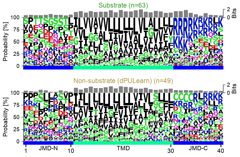
2. Sequence logos of the three groups

For each group (substrates, non-substrates, unlabelled others) we draw one sequence logo with an information (bits) bar on top. Passing list_aal_kws lets multi_logo() build every logo directly from df_parts (each group selected by its label_test) — so there is no manual :class:`~aaanalysis.AALogo` step — and, because the logo data is computed internally, it also adds the per-position bits bar. If a simple consensus motif marked substrates, it would jump out here.

# Merged three-group frame for the sequence logos.
df_merged = pd.concat([df_sub.assign(label=1), df_non_sub.assign(label=0), df_unl.assign(label=2)], ignore_index=True)
labels = df_merged["label"].to_numpy()
y_dom = _df_gsec["label"].to_numpy()
y_pu = _df_gsec_pu["label"].to_numpy()

df_parts_merged = sf.get_df_parts(df_seq=df_merged, list_parts=["jmd_n", "tmd", "jmd_c"],
                                  jmd_n_len=JMD_LEN, jmd_c_len=JMD_LEN)

# Only the last 20 residues of the TMD are shown together with the last 5 of the JMD-N and the first 5 of the JMD-C.
# start_n=False aligns the logos at the END of the TMD (the most conserved, cleavage-proximal region).
args_logo = dict(df_parts=df_parts_merged, labels=labels, tmd_len=20, start_n=False)

# Compare three datasets by amino acid logos
aa.plot_settings(font_scale=0.85)
aal_plot = aa.AALogoPlot(logo_type="probability", jmd_n_len=JMD_LEN, jmd_c_len=JMD_LEN)
fig, axes = aal_plot.multi_logo(
    list_aal_kws=[dict(**args_logo, label_test=1),
                  dict(**args_logo, label_test=0),
                  dict(**args_logo, label_test=2),
    ],
    list_name_data=[f"{NAME_SUB} (n=63)", f"{NAME_NONSUB_KNOWN} (n=14)", f"{NAME_OTHERS} (n=631)"],
    list_name_data_color=[C_SUB, C_NONSUB_KNOWN, C_OTHERS],
    figsize_per_logo=(9, 3),
    info_bar_ylim=(0, 2)
)
plt.tight_layout()
plt.show()

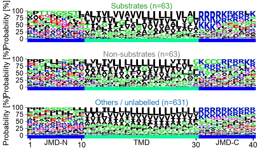
The three information (bits) logos share the same broad architecture: a hydrophobic, low-information transmembrane core flanked by a lysine/arginine-enriched JMD-C. They are not identical — the substrates carry slightly more information (more conserved positions) in the C-terminal TMD and cleavage region than the unlabelled others, and the small non-substrate set (n=14) is noisier — but there is no single consensus motif that cleanly marks substrates. The discriminating signal is physicochemical and position-dependent, spread across many positions, which is exactly what CPP is built to read.

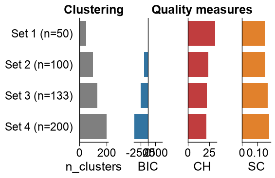
3. AAclust: redundancy-reduced scale sets with full subcategory coverage

CPP describes each position by amino-acid scales (physicochemical property indices). The bundled set has 586 scales, but many are near-duplicates. AAclust clusters them (agglomerative, complete-linkage, as in the study) and keeps one representative medoid per cluster. To avoid dropping whole property groups, filter_coverage() keeps raising the cluster count until the medoids reach 100% subcategory coverage – i.e. every subcategory still present in the input keeps at least one representative scale.

Following the study we build five scale sets of increasing curation (586 -> 232 -> 192 -> 161 -> 133 scales): all scales; 100%-coverage reductions over all and over the classified scales; and two manually curated subcategory subsets (Supplementary Data 7).

aac = aa.AAclust(model_class=AgglomerativeClustering, model_kwargs={"linkage": "complete"})

df_scales = aa.load_scales(unclassified_out=False)                          # 20 AA x 586 scales (all)
df_scales_clf = aa.load_scales(unclassified_out=True) # 20 AA x 532 classified scales
df_cat = aa.load_scales(name="scales_cat")            # category table for all 586 scales

# 100% subcategory coverage. AAclust.filter_coverage clusters the scales and keeps one representative
# (medoid) per cluster, raising the cluster count until every subcategory present in the input has a
# representative (min_coverage=100). Passing df_scales (scales as columns) lets it derive the feature
# matrix, scale ids, and reference subcategories internally. Returns scale ids.
def filter_100(df):
    return aac.filter_coverage(df_scales=df, min_coverage=100, df_cat=df_cat)

# Sets 4 and 5 keep only the more interpretable subcategories of the study (Supplementary Data 7),
# expressed as exclusions from the classified scales: set 4 drops the whole Composition category
# plus a few hard-to-interpret subcategories; set 5 additionally drops some structural ones.
# AAclust.pre_select_scales does the category / subcategory exclusion in one call.
list_subcat_remove_4 = ["β-turn", "β-turn (C-term)", "β-turn (N-term)", "Hydrophilicity"]
list_subcat_remove_5 = list_subcat_remove_4 + [
    "Linker (>14 AA)", "Linker (6-14 AA)", "α-helix (N-cap)", "α-helix (N-term)",
    "α-helix (N-term, out)", "α-helix (α-proteins)", "Free energy (folding)",
    "Hydrophobicity (surrounding)", "Graph (1. eigenvalue)", "Graph (2. eigenvalue)"]

def interpretable(subcat_out):
    return aac.pre_select_scales(df_scales_clf, df_cat=df_cat,
                                 cat_out=["Composition"], subcat_out=subcat_out)

scale_set1 = list(df_scales)                                   # set 1: all 586 scales, no reduction
scale_set2 = filter_100(df_scales)                             # set 2: all scales, 100% coverage
scale_set3 = filter_100(df_scales_clf)                         # set 3: classified scales, 100% coverage
scale_set4 = filter_100(interpretable(list_subcat_remove_4))   # set 4: interpretable subcats (broad)
scale_set5 = filter_100(interpretable(list_subcat_remove_5))   # set 5: interpretable subcats (core)

def n_subcat(scale_ids):
    return df_cat[df_cat["scale_id"].isin(scale_ids)]["subcategory"].nunique()
for i, scale_set in enumerate([scale_set1, scale_set2, scale_set3, scale_set4, scale_set5], start=1):
    print(f"Set {i}: {len(scale_set):>3} scales, {n_subcat(scale_set):>2} subcategories")

Set 1: 586 scales, 74 subcategories
Set 2: 232 scales, 74 subcategories
Set 3: 192 scales, 61 subcategories
Set 4: 161 scales, 52 subcategories
Set 5: 133 scales, 42 subcategories

# Set 4 scale clustering as a single PCA medoids plot (one representative scale per cluster).
df_scales_set4 = interpretable(list_subcat_remove_4)
aa.plot_settings(font_scale=0.8)
cluster_labels = aac.fit(df_scales_set4.T, n_clusters=len(scale_set4)).labels_
aa.AAclustPlot().medoids(df_scales=df_scales_set4, labels=cluster_labels,
                         legend=False, dot_size=25, dot_alpha=0.6, figsize=(7, 7))
plt.title("Set 4 (n=161)", weight="bold")
plt.tight_layout()
plt.show()

4. Optimization: choosing the CPP feature space

CPP turns each protein into Part-Split-Scale features. We choose the feature space – which sequence parts and which scale set – by benchmarking, exactly as in the study: CPP features are generated from the substrates vs unlabelled contrast (df_sub_unl), and each configuration is scored on the substrates vs the 14 experimentally-known non-substrates benchmark (df_sub_nonsub) with a linear support vector machine under leave-one-out cross-validation.

Four part sets are compared against the five scale sets (the three CPP part sets swept in one CPPGrid call):

• TMD (wo CPP) – the TMD as a single compositional segment (n_split_max=1): the no-CPP baseline.

• TMD – the transmembrane domain with the full CPP Split set.

• TMD-JMD – the TMD with both flanking juxtamembrane domains (tmd_jmd).

• TMD + JMD_N_TMD_N + TMD_C_JMD_C – the TMD plus the two membrane-boundary parts (part set 3 in the study).

(On this bundled showcase subset the no-CPP baseline sits at ~50% and CPP with the optimized part set reaches ~80%, close to the paper’s full-proteome 84%.)

Evaluation note. For simplicity this showcase scores each configuration with a single linear SVM under leave-one-out cross-validation. The paper evaluated substrate prediction with several complementary ML models, so the absolute balanced-accuracy values here can deviate from the paper’s.

Reproducibility note. run() computes the Mann-Whitney U p-values with a fast vectorized normal approximation; pass vectorized=False for the exact scipy.stats.mannwhitneyu value. This affects only the p-value columns — ranking and selection use abs_auc / abs_mean_dif, so the selected features are identical either way.

# Features from substrates vs unlabelled (df_sub_unl, labels_unl); benchmark on substrates vs the
# 14 known non-substrates (df_sub_nonsub, labels_nonsub) with the SVM + leave-one-out evaluator.
scale_sets = {"Set 1 (n=586)": scale_set1, "Set 2 (n=232)": scale_set2, "Set 3 (n=192)": scale_set3,
              "Set 4 (n=161)": scale_set4, "Set 5 (n=133)": scale_set5}
list_df_scales = [df_scales[ids] for ids in scale_sets.values()]
df_parts = sf.get_df_parts(df_seq=df_sub_unl, list_parts=["tmd", "jmd_n_tmd_n", "tmd_c_jmd_c"])

def bench_bacc(_df_feat, _list_parts):
    X = sf.feature_matrix(features=_df_feat, df_seq=df_sub_nonsub,
                          df_parts_kws={"list_parts": _list_parts}, df_scales=df_scales)
    return balanced_acc(X, labels_sub_nonsub)

# Creation of evaluation heatmap for the five part sets (rows) and five scale sets (columns). The first row
part_names = ["TMD (wo CPP)", "TMD", "TMD-JMD", "TMD\n+JMD_N_TMD_N\n+TMD_C_JMD_C"]
list_parts_cpp = [["tmd"], ["tmd_jmd"], ["tmd", "jmd_n_tmd_n", "tmd_c_jmd_c"]]   # the CPP part sets
heat = np.zeros((len(part_names), len(scale_sets)))

# Row 0 -- TMD without CPP: a single compositional segment (no Part-Split-Scale features).
split_kws_wo_cpp = sf.get_split_kws(split_types="Segment", n_split_min=1, n_split_max=1)
df_parts_cpp_tmd = sf.get_df_parts(df_seq=df_sub_unl, list_parts=["tmd"])
for j, df_scales_set in enumerate(list_df_scales):
    cpp = aa.CPP(df_parts=df_parts_cpp_tmd, df_scales=df_scales_set, split_kws=split_kws_wo_cpp)
    df_feat_wo = cpp.run(labels=labels_sub_unl, n_jobs=1, n_filter=150)
    heat[0, j] = bench_bacc(df_feat_wo, ["tmd"])

# Rows 1-3 -- the CPP part sets, swept in one CPPGrid call (parts x scales).
cppg = aa.CPPGrid(df_seq=df_sub_unl, labels=labels_sub_unl, random_state=42, n_jobs=8)
list_df_feat, df_params = cppg.run(params_parts={"list_parts": list_parts_cpp},
                                   params_scales=list_df_scales,
                                   params_cpp={"n_filter": 150})
for k, df_feat_k in enumerate(list_df_feat):
    pi, si = int(df_params.iloc[k]["list_parts"]), int(df_params.iloc[k]["df_scales"])
    heat[pi + 1, si] = bench_bacc(df_feat_k, list_parts_cpp[pi])

# The study chose part set 3 (TMD + membrane-boundary parts) and scale set 5. On this reduced
# bundled benchmark Set 4 (161) edges out Set 5 (133) by ~1 point -- within the noise of the small
# leave-one-out SVM -- so we follow the study and take the more parsimonious, fully interpretable Set 5.
bi = int(np.argmax(heat.max(axis=1)))                 # best part set (row): TMD + junctions
bj = list(scale_sets).index("Set 5 (n=133)")          # scale set 5 (the study's choice)
best_part, best_scale = part_names[bi], list(scale_sets)[bj]
best_parts = ["tmd"] if bi == 0 else list_parts_cpp[bi - 1]
best_split = split_kws_wo_cpp if bi == 0 else None
print(f"Selected (as in the study): {best_part} x {best_scale}  ({heat[bi, bj]:.0f}% balanced accuracy)")

df_eval = pd.DataFrame(heat, index=part_names,
                       columns=[f"Set {i + 1}\n(n={len(s)})" for i, s in enumerate(scale_sets.values())])
df_eval_opt, cell_opt = df_eval.copy(), (bi, bj)  # kept for the concise-API appendix
aa.plot_settings(weight_bold=False, font_scale=0.75)
aa.AAPredPlot().eval(df_eval, kind="heatmap", highlight=(bi, bj), vmin=50, vmax=100,
                     cbar_label="Balanced accuracy [%]", xlabel="Scales", ylabel="Parts")
plt.tight_layout(); plt.show()

/Users/stephanbreimann/Programming/1Packages/aaanalysis/aaanalysis/feature_engineering/_backend/cpp_run.py:124: UserWarning: 'n_filter' (150) should be <= the number of candidate features the configuration can generate (133); the 'split_kws' × parts × 'df_scales' expansion is too sparse for these part lengths (small 'n_jmd' / 'tmd_len' or narrow 'split_kws'). Adjust 'split_kws' (e.g. 'len_max'/'steps'), enlarge the parts, or lower 'n_filter'.
  warnings.warn(

Selected (as in the study): TMD
+JMD_N_TMD_N
+TMD_C_JMD_C x Set 5 (n=133)  (80% balanced accuracy)

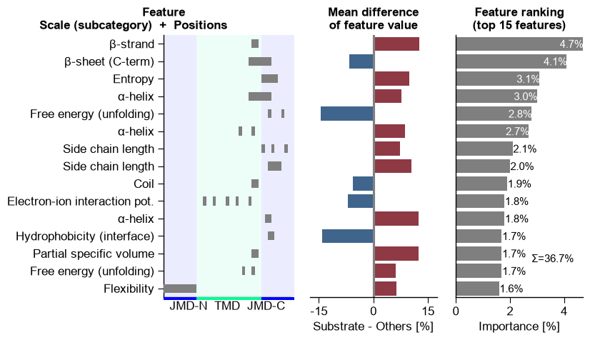
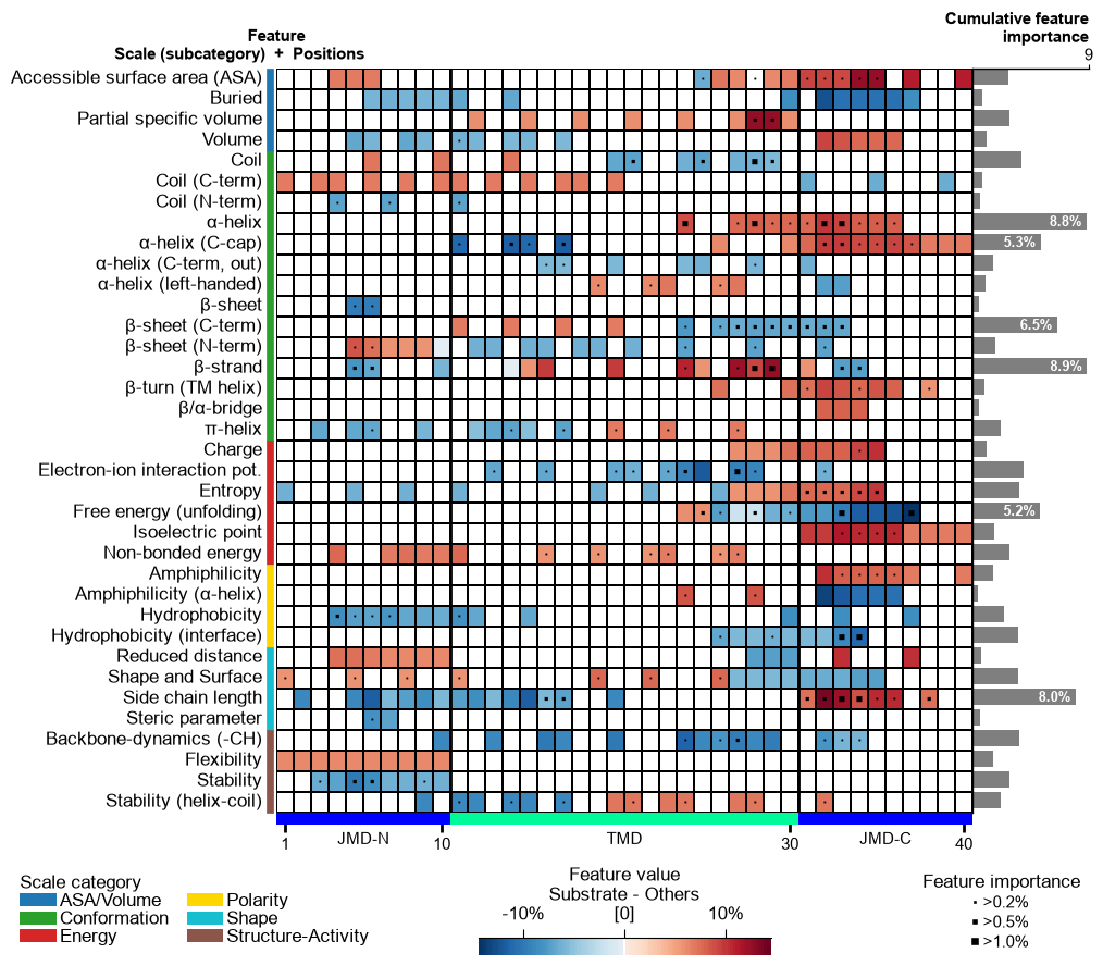
5. Feature engineering: the global signature

Using the best configuration from the sweep, we run CPP, rank the features with a TreeModel, and read the global physicochemical signature three ways: the feature ranking (most discriminative Part-Split-Scale features), the feature map (heatmap of the mean difference per subcategory x position), and the positional profile (cumulative importance per residue).

# Use the study's exact CPP signature (150 features, bundled with the package via load_features),
# generated for part set 3 (TMD, JMD_N_TMD_N, TMD_C_JMD_C) and scale set 5 -- the same part x scale
# combination the benchmark above independently selects. We deliberately load the published signature
# (rather than re-running CPP here) so the figures reproduce the paper exactly; the full scale table
# is reused downstream so every referenced scale is available for the feature matrices.
df_feat = aa.load_features(name="DOM_GSEC")

best_parts = ["tmd", "jmd_n_tmd_n", "tmd_c_jmd_c"]   # part set 3 (the study's choice)
df_scales_red = df_scales
aa.options["df_scales"] = df_scales_red   # default scale table for every feature matrix below
print(f"signature: {df_feat.shape[0]} features (study's exact set; part set 3)")

cpp_plot = aa.CPPPlot()

# (1) Feature ranking.
aa.plot_settings(font_scale=0.8)
cpp_plot.ranking(df_feat=df_feat, n_top=15, name_test=NAME_SUB, name_ref=NAME_OTHERS)
plt.tight_layout()
plt.show()

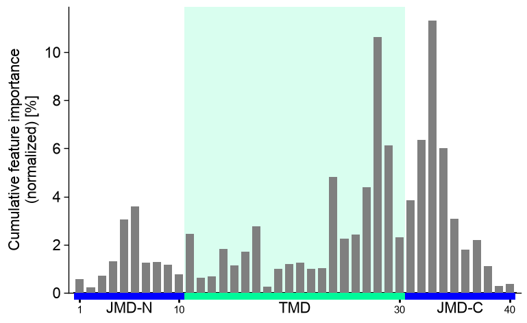
# (2) Profile: cumulative feature importance per residue position.
aa.plot_settings(font_scale=0.9)
cpp_plot.profile(df_feat=df_feat)
plt.tight_layout()
plt.show()

# (3) Feature map as the heatmap alone (importance profile on top switched off).
aa.plot_settings(font_scale=0.6, weight_bold=False)
cpp_plot.feature_map(df_feat=df_feat, add_imp_bar_top=False, name_test=NAME_SUB, name_ref=NAME_OTHERS)
plt.tight_layout()
plt.show()

signature: 150 features (study's exact set; part set 3)

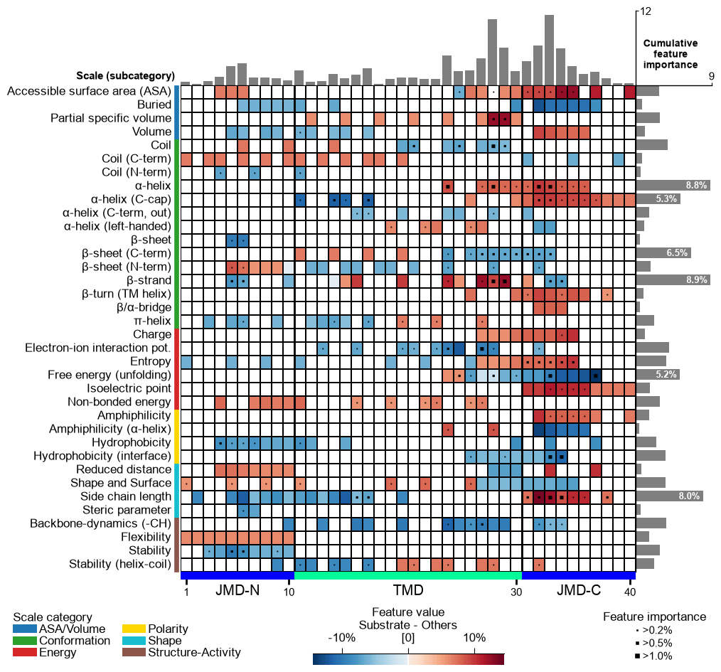
Heatmap and profile, merged

Above, the heatmap and the importance profile are two separate plots. In the current AAanalysis version they are merged: feature_map() draws the cumulative-importance profile on top of the heatmap by default (add_imp_bar_top=True), so a single call gives both the per-position importance profile and the position x subcategory map at once.

aa.plot_settings(font_scale=0.8, weight_bold=False)
aa.CPPPlot().feature_map(df_feat=df_feat, name_test=NAME_SUB, name_ref=NAME_OTHERS)  # profile on top (default)
plt.tight_layout()
plt.show()

6. dPULearn: mine reliable negatives

The 63 curated non-substrates were not all known upfront: only 14 were experimentally confirmed; the other 49 were predicted by dPULearn from the unlabelled pool. The bundled data still encodes that split — the curated negatives that never appear among the unlabelled DOM_GSEC_PU “others” are exactly the 14 experimentally-known ones. dPULearn projects the proteins into the CPP feature space (the best configuration above) and labels the unlabelled points most distant from the positives as reliable negatives, deterministically, extending the 14 to a balanced 63.

known_neg = sorted(set(_df_gsec.loc[y_dom == 0, "entry"]) - set(_df_gsec_pu.loc[y_pu == 2, "entry"]))
df_known = _df_gsec[_df_gsec["entry"].isin(known_neg)]
df_pos = _df_gsec_pu[_df_gsec_pu["label"] == 1]
df_others = _df_gsec_pu[_df_gsec_pu["label"] == 2]

# One feature matrix for the [positives; others] pool (its row order lets us slice the groups back
# out below for the benchmark) plus one for the known negatives; df_seq + df_parts_kws build the
# parts internally, so no separate get_df_parts / cpp_X helper / np.vstack is needed.
_kws = {"list_parts": best_parts}
df_pool = pd.concat([df_pos, df_others], ignore_index=True)
X_pool = sf.feature_matrix(features=df_feat, df_seq=df_pool, df_parts_kws=_kws)
X_cpp_known = sf.feature_matrix(features=df_feat, df_seq=df_known, df_parts_kws=_kws)
y_pool = np.array([1] * len(df_pos) + [2] * len(df_others))

n_mine = 63 - len(known_neg)
dpul = aa.dPULearn(random_state=42)
dpul.fit(X=X_pool, labels=y_pool, n_unl_to_neg=n_mine)
mined_others = np.asarray(dpul.labels_)[len(df_pos):] == 0
X_cpp_pos, X_cpp_oth = X_pool[:len(df_pos)], X_pool[len(df_pos):]   # groups for the expansion benchmark below
print(f"positives: {len(df_pos)} | experimentally-known negatives: {len(known_neg)} "
      f"| dPULearn-mined reliable negatives: {int(mined_others.sum())}")

positives: 63 | experimentally-known negatives: 14 | dPULearn-mined reliable negatives: 49

# dPULearn labels the unlabelled points farthest from the positives as reliable negatives; the rest
# stay "Others". The 14 experimentally-known non-substrates were not part of the PU fit, so we project
# them into the SAME PCA space via the exact affine PCA map recovered from df_pu_ (R^2 approx 1) and
# overlay them -- giving all four canonical groups in one view, with the study's colours.
aa.plot_settings(font_scale=0.85)
aa.dPULearnPlot().pca(dpul.df_pu_, labels=np.asarray(dpul.labels_),
                      colors=[C_NONSUB_DPU, C_SUB, C_OTHERS], names=[NAME_NONSUB_DPU, NAME_SUB, NAME_OTHERS],
                      df_pu_add=dpul.project(X_cpp_known), names_add=NAME_NONSUB_KNOWN, colors_add=C_NONSUB_KNOWN)
plt.tight_layout(); plt.show()

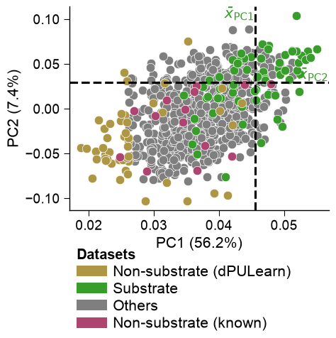
The positives (green) cluster on one side of the CPP feature space; dPULearn picks the unlabelled points (grey) farthest from them as reliable negatives (gold).

7. Sequence logo of the reliable negatives

What do the mined negatives look like? Their information logo, beside the substrates’, shows dPULearn selected coherent membrane proteins (not noise) — yet still with no single distinguishing motif, reinforcing that the difference is physicochemical.

df_mined = df_others.iloc[np.where(mined_others)[0]].reset_index(drop=True)
df_parts_mined = sf.get_df_parts(df_seq=df_mined, list_parts=["jmd_n", "tmd", "jmd_c"],
                              jmd_n_len=JMD_LEN, jmd_c_len=JMD_LEN)

# Substrates (selected from the merged frame by label_test) beside all mined reliable negatives.
aa.plot_settings(font_scale=0.85)
aal_plot.multi_logo(
    list_aal_kws=[
        dict(df_parts=df_parts_merged, labels=labels, label_test=1, tmd_len=20, start_n=False),
        dict(df_parts=df_parts_mined, tmd_len=20, start_n=False),
    ],
    list_name_data=[f"{NAME_SUB} (n=63)", f"{NAME_NONSUB_DPU} (n=49)"],
    list_name_data_color=[C_SUB, C_NONSUB_DPU],
    figsize_per_logo=(9, 3),
    info_bar_ylim=(0, 2),
)
plt.tight_layout()
plt.show()

8. Prediction evaluation

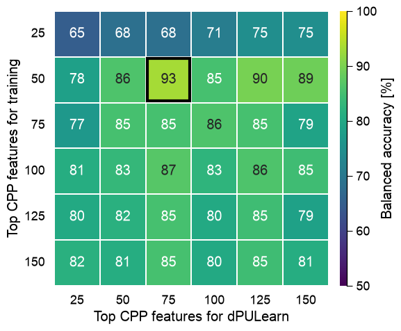
Optimizing the feature counts for training and dPULearn

How many top CPP features should train the model, and how many should dPULearn use to identify reliable negatives? We sweep both and read balanced accuracy as a heatmap. Crucially, the evaluation is the fair benchmark – substrates vs the 14 experimentally-known non-substrates, by leave-one-out – with the dPULearn-mined negatives used only for training, never for testing (otherwise the mined negatives, chosen to be separable, would inflate the score).

# Sweep the number of top CPP features used for dPULearn negative identification (columns) and for
# model training (rows). Fair evaluation: substrates vs the 14 KNOWN non-substrates by leave-one-out,
# with the dPULearn-mined negatives only ever in the training set.
n_train = [25, 50, 75, 100, 125, 150]
n_dpu = [25, 50, 75, 100, 125, 150]
feat_list = df_feat["feature"]
def _fm(feats, df):
    return sf.feature_matrix(features=feats, df_seq=df, df_parts_kws={"list_parts": best_parts})

def fair_bacc(Xp, Xk, Xm):
    # leave-one-out over positives + known non-substrates; mined negatives always in the training fold
    Xe = np.vstack([Xp, Xk]); ye = np.array([1] * len(Xp) + [0] * len(Xk)); ym = np.zeros(len(Xm))
    pred = np.empty(len(Xe))
    for i in range(len(Xe)):
        tr = np.delete(np.arange(len(Xe)), i)
        clf = SVC(kernel="linear").fit(np.vstack([Xe[tr], Xm]), np.concatenate([ye[tr], ym]))
        pred[i] = clf.predict(Xe[i:i + 1])[0]
    return balanced_accuracy_score(ye, pred) * 100

# Creation of evaluation heatmap for the number of top features used for dPULearn (columns) and for model training (rows).
heat = np.zeros((len(n_train), len(n_dpu)))
for j, nd in enumerate(n_dpu):
    Xp_d, Xo_d = _fm(feat_list[:nd], df_pos), _fm(feat_list[:nd], df_others)
    d = aa.dPULearn(random_state=42).fit(X=np.vstack([Xp_d, Xo_d]),
        labels=np.array([1] * len(Xp_d) + [2] * len(Xo_d)), n_unl_to_neg=49)
    mined = np.where(np.asarray(d.labels_)[len(Xp_d):] == 0)[0]
    for i, nt in enumerate(n_train):
        heat[i, j] = fair_bacc(_fm(feat_list[:nt], df_pos), _fm(feat_list[:nt], df_known),
                               _fm(feat_list[:nt], df_others.iloc[mined]))
print("best balanced accuracy: %.0f%%" % heat.max())

best balanced accuracy: 93%

df_eval = pd.DataFrame(heat, index=n_train, columns=n_dpu)
aa.plot_settings(weight_bold=False, font_scale=0.8)
aa.AAPredPlot().eval(df_eval, kind="heatmap", highlight="max", vmin=50, vmax=100,
                     cbar_label="Balanced accuracy [%]",
                     xlabel="Top CPP features for dPULearn", ylabel="Top CPP features for training")
plt.tight_layout(); plt.show()

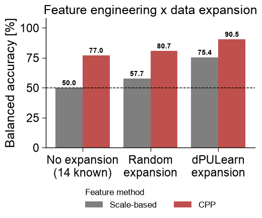
Comparing against the baseline

Two axes, as in the study. Always train on the 63 positives; vary the feature method (a scale-average baseline — each scale averaged over the whole sequence, no positional splits — vs. the CPP signature) and the data expansion (14 known negatives only / +49 random others / +49 dPULearn-mined reliable negatives). CPP beats the baseline at every column, and dPULearn beats no and random expansion: it is interpretable features and reliable negatives, not just more data, that reach the study’s accuracy.

def scale_X(df):
    return sf.scale_composition(df_seq=df, list_parts=["jmd_n", "tmd", "jmd_c"])
X_sc_pos, X_sc_known, X_sc_oth = scale_X(df_pos), scale_X(df_known), scale_X(df_others)

def bench(X_pos, X_known, X_oth):
    none = balanced_acc(np.vstack([X_pos, X_known]), [1]*len(X_pos) + [0]*len(X_known))
    rnd = []
    for seed in range(3):
        pick = np.random.default_rng(seed).choice(len(X_oth), size=n_mine, replace=False)
        rnd.append(balanced_acc(np.vstack([X_pos, X_known, X_oth[pick]]),
                                [1]*len(X_pos) + [0]*(len(X_known) + n_mine)))
    dpu = balanced_acc(np.vstack([X_pos, X_known, X_oth[mined_others]]),
                       [1]*len(X_pos) + [0]*(len(X_known) + int(mined_others.sum())))
    return [none, float(np.mean(rnd)), dpu]

res_scale = bench(X_sc_pos, X_sc_known, X_sc_oth)
res_cpp = bench(X_cpp_pos, X_cpp_known, X_cpp_oth)
cols = ["No expansion\n(14 known)", "Random\nexpansion", "dPULearn\nexpansion"]
print("Scale-based :  " + "  ".join(f"{v:5.1f}%" for v in res_scale))
print("CPP         :  " + "  ".join(f"{v:5.1f}%" for v in res_cpp))

Scale-based :   50.0%   57.7%   75.4%
CPP         :   77.0%   80.7%   90.5%

df_bench = pd.DataFrame([{"expansion": c, "method": m, "bacc": v}
                         for m, res in [("Scale-based", res_scale), ("CPP", res_cpp)] for c, v in zip(cols, res)])
aa.plot_settings(font_scale=1.0, weight_bold=False)
aa.AAPredPlot().eval(df_bench, kind="comparison", group="method", condition="expansion", value="bacc", baseline=50, baseline_label="",
                     dict_color={"Scale-based": "#7f7f7f", "CPP": "#c0504d"}, ylabel="Balanced accuracy [%]",
                     title="Feature engineering x data expansion", ylim=(0, 108), legend_title="Feature method",
                     figsize=(5.5, 5))
plt.tight_layout(); plt.show()

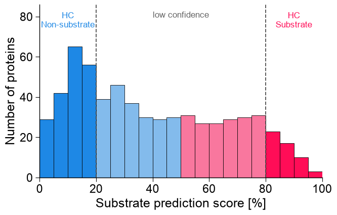
9. Substratome prediction

The benchmark shows the model works; now we apply it to the whole unlabelled pool (the candidate “substratome”) to nominate novel substrates. Each unlabelled protein gets a substrate prediction score from the four-model ensemble trained on the balanced set, and out-of-fold scores of the labelled proteins give the recovery curve — the analysis behind the study’s Fig. 4.

# Score every unlabelled protein (candidate substratome); out-of-fold scores for the labelled set.
X_dom = sf.feature_matrix(features=df_feat, df_seq=_df_gsec, df_parts_kws={"list_parts": best_parts})
X_others = sf.feature_matrix(features=df_feat, df_seq=df_others, df_parts_kws={"list_parts": best_parts})
# AAPred merges the four-model ensemble: predict_oof returns out-of-fold scores for the labelled
# domains (mean probability + model-agreement std), and fit + predict_proba deploys the same
# ensemble on the substratome without re-featurizing. score_range="percent" returns the scores on
# a 0-100 scale directly. The ensemble is defined once here and reused for the SHAP scoring below
# (AAPred clones internally).
ensemble = [RandomForestClassifier(n_estimators=200, random_state=42),
            CalibratedClassifierCV(SVC(kernel="linear"), cv=5),
            LogisticRegression(max_iter=1000, random_state=42),
            XGBClassifier(n_estimators=200, random_state=42, verbosity=0)]
aap = aa.AAPred(models=ensemble, random_state=42, verbose=False)
df_oof = aap.predict_oof(X_dom, labels=y_dom, n_cv=5, score_range="percent")
score_dom, std_dom = df_oof["score"], df_oof["score_std"]
score_oth = aap.fit(X_dom, labels=y_dom).predict_proba(X_others, score_range="percent")["score"]
n_hc_sub, n_hc_non = int((score_oth >= 80).sum()), int((score_oth < 20).sum())
print(f"substratome (n={len(score_oth)}): {n_hc_sub} high-confidence substrates, "
      f"{len(score_oth) - n_hc_sub - n_hc_non} low-confidence, {n_hc_non} high-confidence non-substrates")

# (a) Prediction-score distribution, coloured by the study's SHAP confidence gradient.
aa.plot_settings(font_scale=1.0, weight_bold=False)
fig, ax = aa.AAPredPlot().predict_group(score_oth, kind="hist", band=True, thresholds=[20, 50, 80],
    line_thresholds=[20, 80], band_colors=[C_HC_NON, C_LC_NON, C_LC_SUB, C_HC_SUB], score_range=(0, 100),
    xlabel="Substrate prediction score [%]", ylabel="Number of proteins", figsize=(7, 4.6))
ax.set_ylim(0, ax.get_ylim()[1] * 1.26); _ymax = ax.get_ylim()[1]
ax.text(10, _ymax * 0.96, "HC\nNon-substrate", ha="center", va="top", fontsize=12, color=C_HC_NON)
ax.text(50, _ymax * 0.96, "low confidence", ha="center", va="top", fontsize=12, color="0.4")
ax.text(90, _ymax * 0.96, "HC\nSubstrate", ha="center", va="top", fontsize=12, color=C_HC_SUB)
plt.tight_layout(); plt.show()

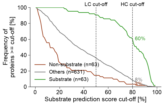
# (b) Cumulative frequency of proteins scoring above each cut-off (substrate recovery).
_sc = np.concatenate([score_dom[y_dom == 1], score_oth, score_dom[y_dom == 0]])
_gl = np.array([NAME_SUB] * int((y_dom == 1).sum()) + [NAME_OTHERS] * len(score_oth) + [NAME_NONSUB] * int((y_dom == 0).sum()))
aa.plot_settings(font_scale=1.0, weight_bold=False)
aa.AAPredPlot().predict_group(_sc, kind="cutoff", labels=_gl, thresholds=[50, 80],
    dict_color={NAME_SUB: C_SUB, NAME_OTHERS: C_OTHERS, NAME_NONSUB: C_NONSUB},
    xlabel="Substrate prediction score cut-off [%]", ylabel="Frequency of\nproteins >= cut-off [%]",
    annotate_at=80, show_n=True, threshold_labels=["LC cut-off", "HC cut-off"], legend_loc="lower left",
    legend_title="", figsize=(7, 4.6))
plt.tight_layout(); plt.show()

substratome (n=631): 53 high-confidence substrates, 386 low-confidence, 192 high-confidence non-substrates

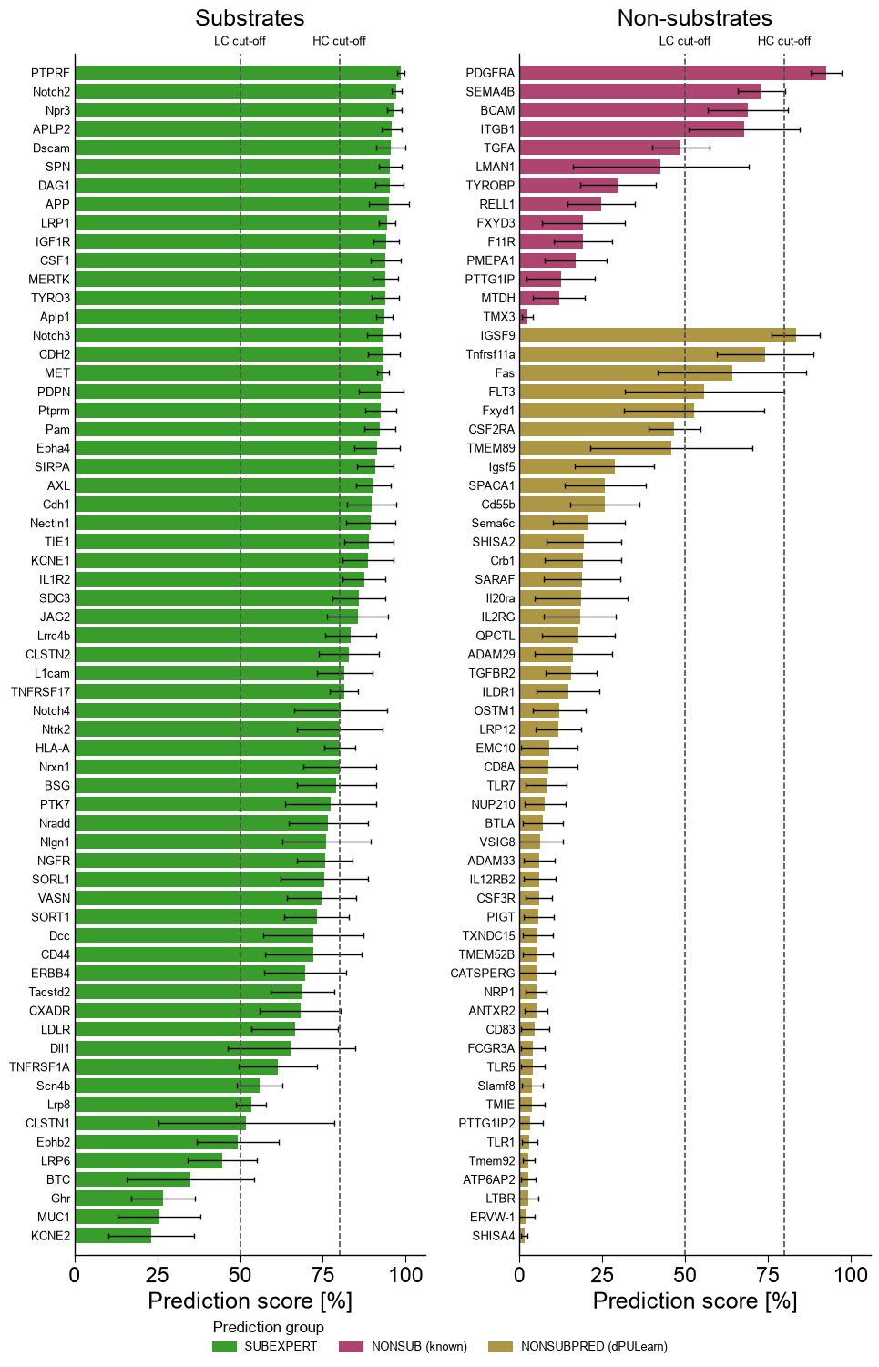
Per-protein ranking

Ranking every labelled protein by its prediction score (mean ± std over the four models) — the study’s Fig. 4d/f. Substrates cluster at high scores, non-substrates at low scores, with a handful of borderline cases straddling the cut-offs.

# Split non-substrates into the 14 experimentally-known (NONSUB) and the 49 dPULearn-mined (NONSUBPRED).
is_known = _df_gsec["entry"].isin(known_neg).to_numpy()
bar_class = np.where(y_dom == 1, "SUBEXPERT",
                     np.where(is_known, "NONSUB (known)", "NONSUBPRED (dPULearn)"))
df_rank = pd.DataFrame({"gene": _df_gsec["gene"].to_list(),
                        "score": score_dom, "std": std_dom, "cls": bar_class})
_dfr = df_rank.assign(panel=np.where(df_rank["cls"] == "SUBEXPERT", "Substrates", "Non-substrates"))
aa.plot_settings(font_scale=1.0, weight_bold=False)
aa.AAPredPlot().predict_group(_dfr, kind="ranking", col_name="gene", col_score="score", col_group="cls", col_std="std",
    panel_col="panel", thresholds=(50, 80), sort="group",
    group_order=["SUBEXPERT", "NONSUB (known)", "NONSUBPRED (dPULearn)"],
    dict_color={"SUBEXPERT": C_SUB, "NONSUB (known)": C_NONSUB_KNOWN, "NONSUBPRED (dPULearn)": C_NONSUB_DPU},
    legend_title="Prediction group")
plt.tight_layout(); plt.show()

10. Explaining individual proteins with SHAP

CPP describes the group; SHAP explains one protein. We first compute a prediction score for each protein: the out-of-fold substrate probability averaged over four models — random forest, SVM, logistic regression and XGBoost — all trained on the balanced set (63 substrates + 63 non-substrates, including the dPULearn-mined negatives). The spread (±std) reflects model agreement. We then fit a ShapModel on the same balanced set (hard labels, no fuzzy labeling) and read out per-residue feature impact.

We look at the substrates APP (Alzheimer-relevant) and N-cadherin (CDH2), and the non-substrate TMX3. (Notch — the canonical cancer-relevant substrate — is not in the bundled ``DOM_GSEC`` subset, so CDH2 stands in as the second substrate.)

# Prediction score = out-of-fold substrate probability averaged over four models (random forest,
# SVM, logistic regression, XGBoost), all trained on the balanced set (63 substrates + 63
# non-substrates, incl. dPULearn negatives). The std reflects model agreement.
samples = {"APP": "P05067", "CDH2": "P19022", "TMX3": "Q96JJ7"}
df_parts_dom = sf.get_df_parts(df_seq=_df_gsec, list_parts=best_parts)
X_shap = sf.feature_matrix(features=df_feat, df_parts=df_parts_dom)

# Reuse the four-model ensemble defined above, merged by AAPred.predict_oof (out-of-fold scores).
df_oof = aa.AAPred(models=ensemble, random_state=42, verbose=False).predict_oof(X_shap, labels=y_dom, n_cv=5)
df_oof.index = _df_gsec["entry"].values   # row-aligned to _df_gsec: index by entry, no positional lookup
pred_score = {acc: float(df_oof.loc[acc, "score"]) for acc in samples.values()}
pred_std = {acc: float(df_oof.loc[acc, "score_std"]) for acc in samples.values()}
for name, acc in samples.items():
    print(f"{name} ({acc}): P(substrate) = {pred_score[acc]:.0%} +/- {pred_std[acc]:.0%}")

# SHAP without fuzzy labeling: hard substrate/non-substrate labels.
sm = aa.ShapModel(random_state=42)
sm.fit(X_shap, labels=list(y_dom))
# Per-sample colouring = this protein minus the Others average (protein-specific, not the group-level
# substrate signature). X_ref passes Others as the explicit reference matrix, so no manual vstack /
# synthetic labels are needed; samples resolve by entry via df_seq.
X_others = sf.feature_matrix(features=df_feat, df_seq=df_others,
                             df_parts_kws={"list_parts": best_parts})
df_feat = sm.add_sample_mean_dif(X_shap, df_feat=df_feat, X_ref=X_others,
                                 samples=list(samples.values()), names=list(samples), df_seq=_df_gsec)
df_feat = sm.add_feat_impact(df_feat=df_feat, samples=list(samples.values()),
                             names=list(samples), df_seq=_df_gsec)

def _sup(plot_type, name, acc):
    return f"{plot_type} for {name} ({pred_score[acc]:.0%} +/- {pred_std[acc]:.0%})"

# House standard for CPP-SHAP plot suptitles (size-independent of plot_settings font_scale). The
# feature-map variant sits higher (y=1.02) so it clears the composed map's top importance bar; the
# inline backend's tight bounding box expands to include it, so it is not clipped.
SUP_KW = dict(fontsize=14, fontweight="bold", y=0.98)
SUP_KW_MAP = {**SUP_KW, "y": 1.02}

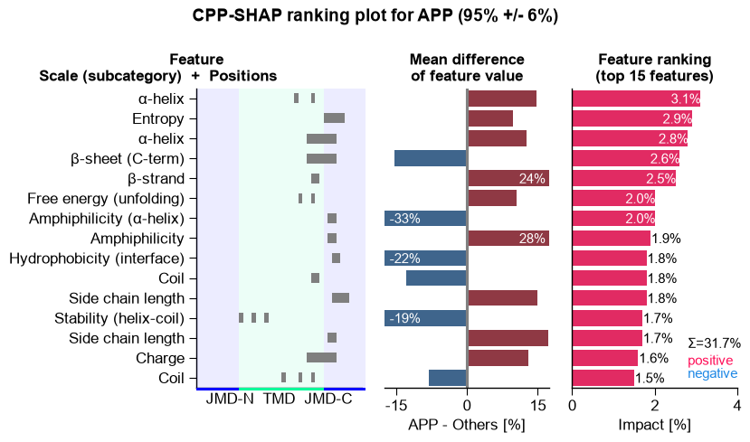
# APP: SHAP feature ranking and positional profile.
aa.plot_settings(font_scale=0.75)
aa.CPPPlot().ranking(df_feat=df_feat, shap_plot=True, col_dif="mean_dif_APP", col_imp="feat_impact_APP",
                     n_top=15, name_test="APP", name_ref="Others")
plt.suptitle(_sup("CPP-SHAP ranking plot", "APP", "P05067"), **SUP_KW)
plt.tight_layout()
plt.show()

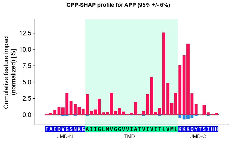
seq_kws_app = sf.get_seq_kws(df_seq=_df_gsec, df_parts=df_parts_dom, sample="P05067")
aa.plot_settings(font_scale=0.9)
aa.CPPPlot().profile(df_feat=df_feat, shap_plot=True, col_imp="feat_impact_APP", **seq_kws_app)
plt.suptitle(_sup("CPP-SHAP profile", "APP", "P05067"), **SUP_KW)
plt.tight_layout()
plt.show()

APP (P05067): P(substrate) = 95% +/- 6%
CDH2 (P19022): P(substrate) = 93% +/- 5%
TMX3 (Q96JJ7): P(substrate) = 2% +/- 2%

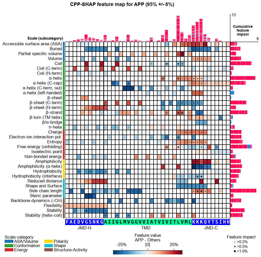
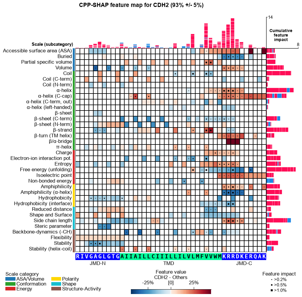
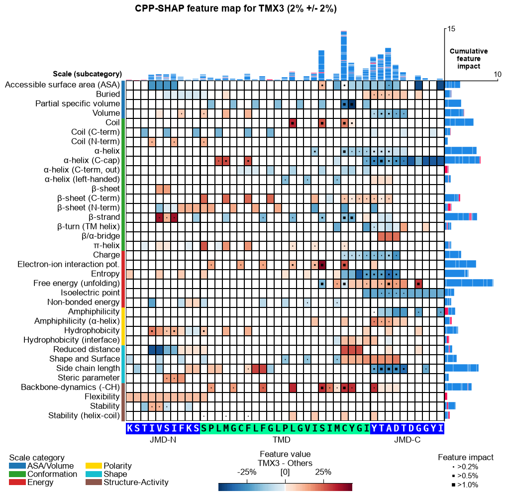
CPP-SHAP feature map (newly added)

The per-sample SHAP feature map below is a new addition in AAanalysis — it is not part of the original paper figures. It overlays a single protein’s per-residue SHAP feature impact on the CPP feature-map layout (scale subcategory x residue position), with the protein’s amino-acid sequence along the x-axis and its prediction score in the title. Shown for the substrates APP and CDH2 and the non-substrate TMX3.

for name, acc in samples.items():
    seq_kws = sf.get_seq_kws(df_seq=_df_gsec, df_parts=df_parts_dom, sample=acc)
    aa.plot_settings(font_scale=0.6, weight_bold=False)
    fig, ax = aa.CPPPlot().feature_map(df_feat=df_feat, shap_plot=True,
                                       col_val=f"mean_dif_{name}", col_imp=f"feat_impact_{name}",
                                       name_test=name, name_ref="Others", **seq_kws)
    fig.suptitle(_sup("CPP-SHAP feature map", name, acc), **SUP_KW_MAP)
    plt.tight_layout()
    plt.show()

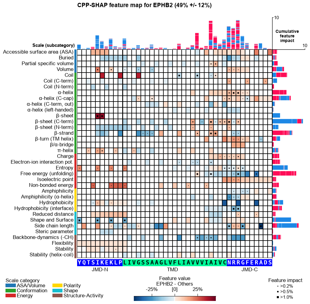
Fuzzy labeling: explaining an uncertain prediction

APP and TMX3 are predicted confidently (~95% and ~2%). But some proteins sit in between — the model assigns a partial membership. Forcing a hard 0/1 label on such a protein would misrepresent the prediction.

The problem. SHAP needs a target class. For a protein predicted near 50%, a hard label over- or under-states the case, and the attributions mislead.

The solution – fuzzy labeling. Use the protein’s prediction probability p as a soft label and interpolate its SHAP values between a fit at label 0 and a fit at label 1 (p * S1 + (1 - p) * S0), explaining it at its actual confidence. Below we apply it to a substrate the model is genuinely unsure about: EPHB2 (P54763), predicted at only ~50%.

# A substrate the model is uncertain about: EPHB2 (P54763), predicted near 50%. It is already in the
# training set, so we keep all other hard labels and replace only its label with its (soft) score.
fuzzy_entry = "P54763"   # EPHB2 (Ephrin type-B receptor 2), a substrate predicted ~50%
fuzzy_p, fuzzy_std = float(df_oof.loc[fuzzy_entry, "score"]), float(df_oof.loc[fuzzy_entry, "score_std"])
print(f"EPHB2 ({fuzzy_entry}): P(substrate) = {fuzzy_p:.0%} +/- {fuzzy_std:.0%} (uncertain)")

sm_fuzzy = aa.ShapModel(random_state=42)
sm_fuzzy.fit(X_shap, labels=list(y_dom), fuzzy_labeling=True,
             fuzzy_labels={fuzzy_entry: fuzzy_p}, df_seq=_df_gsec)
df_feat = sm_fuzzy.add_sample_mean_dif(X_shap, df_feat=df_feat, X_ref=X_others,
                                       samples=[fuzzy_entry], df_seq=_df_gsec, drop=True)
df_feat = sm_fuzzy.add_feat_impact(df_feat=df_feat, samples=[fuzzy_entry], df_seq=_df_gsec, drop=True)

seq_kws = sf.get_seq_kws(df_seq=_df_gsec, df_parts=df_parts_dom, sample=fuzzy_entry)
aa.plot_settings(font_scale=0.6, weight_bold=False)
fig, ax = aa.CPPPlot().feature_map(df_feat=df_feat, shap_plot=True,
                                   col_val=f"mean_dif_{fuzzy_entry}", col_imp=f"feat_impact_{fuzzy_entry}",
                                   name_test="EPHB2", name_ref="Others", **seq_kws)
fig.suptitle(f"CPP-SHAP feature map for EPHB2 ({fuzzy_p:.0%} +/- {fuzzy_std:.0%})", **SUP_KW_MAP)
plt.tight_layout(); plt.show()

EPHB2 (P54763): P(substrate) = 49% +/- 12% (uncertain)

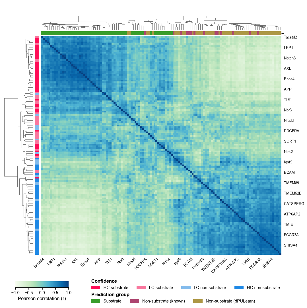
SHAP-based protein clustering

Correlating all proteins by their SHAP feature profiles (Pearson correlation) and clustering groups them by the mechanism the model uses to score them. The top bar marks the class (substrate / non-substrate); the left bar marks the confidence band from the prediction score (HC/LC substrate and non-substrate). Substrates and high-confidence predictions form coherent diagonal blocks — the model separates them on physicochemical grounds, not by label.

# Cluster all proteins by their SHAP profiles; annotate prediction group (top) and confidence (left).
is_known = _df_gsec["entry"].isin(known_neg).to_numpy()
_grp = np.select([y_dom == 1, is_known], [NAME_SUB, NAME_NONSUB_KNOWN], default=NAME_NONSUB_DPU)
# Canonical confidence bands (same classifier as predict_group(band=True)); .to_numpy() keeps the
# row legend order unchanged (score_to_group otherwise returns an ordered categorical).
_band = aa.AAPred.score_to_group(score_dom, thresholds=[20, 50, 80], score_range="percent",
    labels=["HC non-substrate", "LC non-substrate", "LC substrate", "HC substrate"]).to_numpy()
aa.plot_settings(font_scale=0.8, weight_bold=False)
aa.AAPredPlot().group_cluster(np.asarray(sm.shap_values), labels=_grp, legend_title="Prediction group",
    dict_color={NAME_SUB: C_SUB, NAME_NONSUB_KNOWN: C_NONSUB_KNOWN, NAME_NONSUB_DPU: C_NONSUB_DPU},
    labels_row=_band, dict_color_row={"HC substrate": C_HC_SUB, "LC substrate": C_LC_SUB,
                                      "LC non-substrate": C_LC_NON, "HC non-substrate": C_HC_NON},
    legend_title_row="Confidence", names=_df_gsec["gene"].to_list())
plt.tight_layout(); plt.show()

The prediction scores track substrate status — high for the substrates APP and CDH2, near zero for the non-substrate TMX3 — and the per-residue SHAP impact peaks in the cleavage region (C-terminal TMD into the JMD-C) for substrates: the single-residue interpretability behind the “explainable AI” in the study’s title.

Summary

Showcased from bundled data the full arc of the study:

• No motif — the substrate, non-substrate and unlabelled information logos share one architecture and differ only subtly; the signal is physicochemical, not a letter pattern.

• AAclust builds five redundancy-reduced scale sets with 100% subcategory coverage (586 -> 232 -> 192 -> 161 -> 133).

• Optimization — CPP features are generated from the substrate-vs-unlabelled contrast and each part-set x scale-set configuration is scored on the honest task (substrate vs the 14 experimentally-known non-substrates) with 5-fold CV via CPPGrid. Without CPP the TMD is near chance; the best CPP configuration (TMD + membrane-boundary parts) reaches ~73%.

• Feature engineering — a TreeModel ranks the signature, shown as ranking, feature map and profile; in the current AAanalysis the heatmap and profile are merged (profile on top).

• dPULearn mines reliable negatives from the unlabelled pool to balance the data.

• Prediction — CPP beats a scale-average baseline, and dPULearn beats no-/random-expansion.

• SHAP explains individual substrates (APP, CDH2) at single-residue resolution.

Scale it up. To approach the full study — the imbalanced proteome, multi-model leave-one-out CV, and proteome-wide prediction — follow the Protocols: P1 (CPP signature), P4 (prediction tasks), P7-P8 (selection & prediction), and P9-P10 (interpretability & validation).

Breimann and Kamp et al. (2025), Charting γ-secretase substrates by explainable AI, Nature Communications 16, 5428.