aaanalysis.AAclustPlot.eval

static AAclustPlot.eval(df_eval=None, figsize=(6, 4), dict_xlims=None)

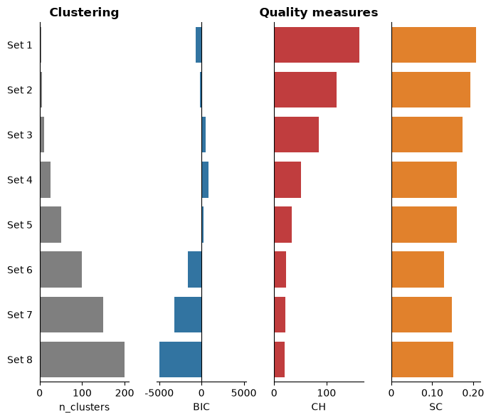
Plots evaluation of n_clusters and clustering metrics BIC, CH, and SC from df_seq.

The clustering evaluation metrics (BIC, CH, and SC) are ranked by the average of their independent rankings.

Parameters:

• df_eval (pd.DataFrame, shape (n_datasets, n_metrics)) –

  DataFrame with evaluation measures for scale sets. Each row corresponds to a specific scale set and columns are as follows:

  • ’name’: Name of clustering datasets.

  • ’n_clusters’: Number of clusters.

  • ’BIC’: Bayesian Information Criterion.

  • ’CH’: Calinski-Harabasz Index.

  • ’SC’: Silhouette Coefficient.

• figsize (tuple, default=(7, 6)) – Figure dimensions (width, height) in inches.

• dict_xlims (dict, optional) – A dictionary containing x-axis limits for subplots. Keys should be the subplot axis number ({0, 1, 2, 4}) and values should be tuple specifying (xmin, xmax). If None, x-axis limits are auto-scaled.

Returns:

• fig (plt.Figure) – Figure object for evaluation plot

• axes (array of plt.Axes) – Array of Axes objects, each representing a subplot within the figure.

Notes

• The data is ranked in ascending order of the average ranking of the scale sets.

See also

• AAclust.eval() for details on evaluation measures.

Examples

To demonstrate the AAclustPlot().eval() method, we create an example dataset:

from sklearn.decomposition import PCA
import matplotlib.pyplot as plt
import aaanalysis as aa
aa.options["verbose"] = False
# Obtain example scale dataset
df_scales = aa.load_scales()
X = df_scales.T
# Fit AAclust model and retrieve labels for evaluation
aac = aa.AAclust()
list_labels = [aac.fit(X, n_clusters=n).labels_ for n in [3, 5, 10, 25, 50, 100, 150, 200]]
df_eval = aac.eval(X, list_labels=list_labels)

And can visualize now all results of the `df_eval``. The clustering results are ranked in from top to down by the average ranking over all three quality measures (BIC, SC, and CH):

aac_plot = aa.AAclustPlot(model_class=PCA)
fig, ax = aac_plot.eval(df_eval=df_eval)
plt.show()

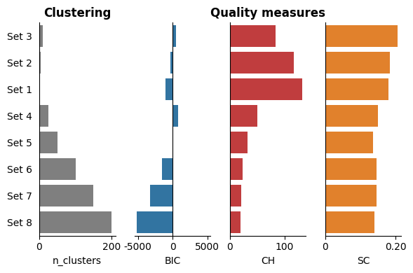
You can adjust the x-axis limits of the three quality measures using the dict_xlims parameter:

dict_xlims = {0:(0, 250), 1:(-7500, 7500), 2:(0, 200), 3:(0, 0.4)}
aac_plot.eval(df_eval=df_eval, dict_xlims=dict_xlims)
plt.show()