dPULearn.project

dPULearn.project(X, method='lstsq')

Project new samples into the fitted PCA coordinate space (the PCi columns of df_pu_).

After PCA-based fitting, this maps held-out samples from the same feature space into the principal-component coordinates learned during dPULearn.fit(), so new proteins can be placed alongside the identified negatives (e.g. overlaying an extra group in dPULearnPlot.pca()).

Because dPULearn fits Principal Component Analysis (PCA) on the transposed feature matrix (PCA().fit(X.T)), there is no exact out-of-sample forward transform; instead a linear map is reconstructed from the fit pairs (X, df_pu_). Both methods reproduce df_pu_ on the fitted samples (when n_features >= n_samples) and are therefore exact on the fit pool and an approximation for genuinely new samples. Deterministic (no randomness).

Added in version 1.1.0.

Parameters:

• X (array-like, shape (n_new_samples, n_features)) – Feature matrix of the samples to project. Must have the same number of features (columns) as the matrix used in dPULearn.fit().

• method ({'lstsq', 'components'}, default='lstsq') –

  Projection map reconstructed from the fitted (X, df_pu_) pairs (both exact on the fit pool, differing only for genuinely new samples):

  • lstsq: affine least-squares map ([X | 1] -> df_pu_), the minimum-norm solution. Reproduces the hand-rolled projection used in the use case.

  • components: exact PCA-geometry map. Row-centers each sample by its own feature mean, then applies the minimum-norm linear map, which equals the fitted PCA’s U @ inv(Sigma) restricted to the stored components.

Returns:

df_proj – Projected coordinates with the same PCi value columns as df_pu_ (in the same order), so it can be passed directly to dPULearnPlot.pca() as an extra group.

Return type:

pd.DataFrame, shape (n_new_samples, n_pcs)

Notes

• Only available after PCA-based identification (fit with metric=None); distance-based identification produces no principal components to project into.

• The projection is exact for the samples used in fit and interpolates for new samples, so points far from the fitted distribution should be interpreted with care.

See also

• dPULearn.fit() for the identification that defines the PC space.

• dPULearnPlot.pca() for overlaying projected groups on the PCA plot.

Examples

After a PCA-based fit, dPULearn().project() maps held-out samples from the same feature space into the fitted principal-component coordinates (the PCi columns of df_pu_). This lets you place new proteins alongside the identified negatives, for example to overlay an additional group in the PCA plot. We load an example dataset, hold out a few proteins, and fit dPULearn on the rest:

import numpy as np
import matplotlib.pyplot as plt
import aaanalysis as aa
aa.options["verbose"] = False
# γ-secretase substrates (positives) + proteins with unknown status (unlabeled)
df_seq = aa.load_dataset(name="DOM_GSEC_PU")
labels_all = df_seq["label"].to_numpy()
df_feat = aa.load_features(name="DOM_GSEC")
sf = aa.SequenceFeature()
X = sf.feature_matrix(features=df_feat["feature"], df_parts=sf.get_df_parts(df_seq=df_seq))
# Hold out 10 proteins to project after fitting; fit dPULearn on the rest
rng = np.random.default_rng(0)
mask_new = np.zeros(len(X), dtype=bool)
mask_new[rng.choice(len(X), size=10, replace=False)] = True
X_fit, labels_fit, X_new = X[~mask_new], labels_all[~mask_new], X[mask_new]
n_pos = int((labels_fit == 1).sum())
dpul = aa.dPULearn().fit(X_fit, labels=labels_fit, n_neg=n_pos)

Pass the held-out feature matrix to project() to obtain their coordinates in the fitted PC space. The returned DataFrame carries the same PCi columns as dPULearn().df_pu_:

df_proj = dpul.project(X_new)
aa.display_df(df_proj, n_rows=10, show_shape=True)

DataFrame shape: (10, 7)

	PC1 (56.0%)	PC2 (7.4%)	PC3 (2.9%)	PC4 (2.8%)	PC5 (2.1%)	PC6 (1.7%)	PC7 (1.6%)
1	0.043861	-0.017151	0.009517	0.080963	0.068627	0.014991	0.022464
2	0.047893	0.016042	-0.024519	-0.004018	0.017070	-0.020411	-0.038839
3	0.047519	0.031883	-0.022193	0.033516	0.022347	-0.033253	-0.026722
4	0.039927	-0.045211	-0.047730	0.029938	0.022512	-0.019787	-0.021570
5	0.045709	0.012006	0.010413	0.034537	-0.045231	0.014827	-0.024091
6	0.043690	-0.028165	-0.065779	0.050376	0.035807	0.006461	-0.011233
7	0.042007	-0.026123	-0.050801	0.013587	-0.016452	-0.023217	-0.040908
8	0.031670	-0.021102	0.012709	0.018437	0.023056	0.075416	0.057489
9	0.042825	-0.034355	0.031250	0.041629	0.000038	0.059496	-0.010246
10	0.046230	-0.029815	-0.003327	0.039344	-0.014050	-0.001047	-0.004704

The method parameter selects how the feature-space to PC-space map is reconstructed. Both methods reproduce df_pu_ on the fitted samples (exact on the fit pool) and interpolate for new samples, differing only off the fit pool: 'lstsq' (default) is the affine least-squares map, and 'components' the exact PCA-geometry map:

for method in ["lstsq", "components"]:
    df_m = dpul.project(X_new, method=method)
    print(method, "->", df_m.shape, "| PC1 range:",
          round(df_m.iloc[:, 0].min(), 3), "to", round(df_m.iloc[:, 0].max(), 3))

lstsq -> (10, 7) | PC1 range: 0.032 to 0.048
components -> (10, 7) | PC1 range: 0.032 to 0.048

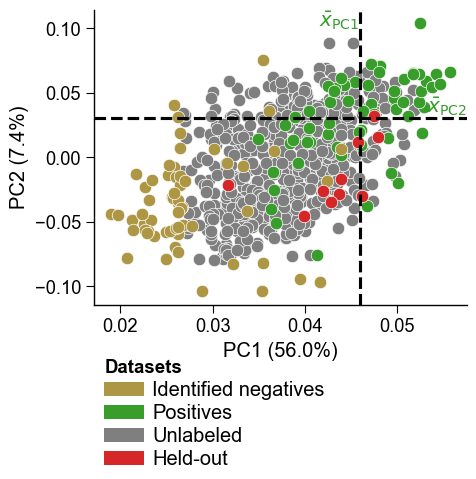
The projected coordinates can be overlaid on the PCA plot as an additional group via dPULearnPlot().pca(df_pu_add=...) (see the dPULearnPlot.pca example for details):

aa.plot_settings(font_scale=0.8)
aa.dPULearnPlot().pca(df_pu=dpul.df_pu_, labels=dpul.labels_,
                      df_pu_add=df_proj, names_add="Held-out", colors_add="tab:red")
plt.tight_layout()
plt.show()