AAclust: Selecting redundancy-reduced scale sets

The Amino Acid clustering (AAclust) class is k-optimized clustering wrapper for selecting redundancy-reduced sets of numerical scales, introduced in [Breimann24a].

We load an example scale dataset to showcase it:

import aaanalysis as aa
aa.options["verbose"] = False

# Create test dataset of 25 amino acid scales
df_scales = aa.load_scales()
X = df_scales.T

AAclust can utilize any clustering model that uses the n_clusters parameter:

from sklearn.cluster import KMeans

# AAclust with KMens (default)
aac = aa.AAclust(model_class=KMeans)

By fitting AAclust, its three-step algorithm is performed to select an optimized n_clusters (k). The three steps involve (1) an estimation of lower bound of k, (2) refinement of k, and (3) an optional clustering merging. Various results are saved as attributes:

# Fit clustering model (KMeans by default)
aac = aa.AAclust()
aac.fit(X)
# Get output parameters
n_clusters = aac.n_clusters
print("n_clusters: ", n_clusters)

n_clusters:  48

Instead of optimizing the number of clusters, we can pre-defined it using the n_clusters parameter:

# Fit clustering model with pre-selected k
labels = aac.fit(X, n_clusters=5).labels_

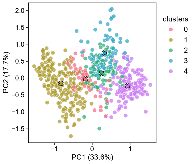
We can visualize the clustering results and the obtained cluster centers using the respective plotting AAclustPlot class. For scales, pass the scales DataFrame directly via df_scales — it is transposed internally, so you never call .T yourself. All data points are shown in the PCA plot with the cluster centers highlighted by an ‘x’:

import matplotlib.pyplot as plt

aac_plot = aa.AAclustPlot()
aa.plot_settings()
fig, ax = aac_plot.centers(df_scales=df_scales, labels=labels)
plt.tight_layout()
plt.show()

To obtain redundancy-reduced scale sets, AAclust selects one medoid per cluster, which is the scale closest to center of the respective cluster. These can be highlighted using the AAclustPlot.medoids method

aac_plot = aa.AAclustPlot()
aa.plot_settings()
fig, ax = aac_plot.medoids(df_scales=df_scales, labels=labels)
plt.tight_layout()
plt.show()

A one-call shortcut: select_scales

The fit → medoid → map-back-to-columns sequence above is the canonical scale-selection workflow, so AAclust bundles it into a single call. select_scales clusters the scales in df_scales and returns the columns of the representative (medoid) scales — one per cluster — without the manual transpose and medoid-name bookkeeping. The fitted attributes (labels_, medoid_names_, …) remain available on the instance afterwards.

# One-call redundancy reduction: return the representative (medoid) scale per cluster
df_scales_selected = aac.select_scales(df_scales, n_clusters=100)
aa.display_df(df_scales_selected, n_rows=10, show_shape=True)

DataFrame shape: (20, 100)

	ROBB760108	SIMZ760101	ARGP820102	KANM800103	CORJ870105	GUYH850101	BIGC670101	ROSG850102	ZIMJ680105	RADA880102	MIYS990101	COHE430101	BLAM930101	KARS160108	BUNA790103	ROBB760101	PONP800102	FASG760101	BAEK050101	CHAM830101	QIAN880123	ROBB760106	LEVM760105	CHAM830107	CHAM830108	JANJ780101	CHOC760103	CHOP780204	QIAN880109	QIAN880114	LEVM780102	CHOP780211	CHOP780214	CHOP780213	ROBB760111	LEVM780106	CIDH920105	DAYM780101	DAYM780201	WOLR790101	BLAS910101	PRAM900101	AURR980119	ISOY800102	FAUJ880108	LINS030112	FAUJ880111	FAUJ880112	ISOY800101	ONEK900102	ZIMJ680104	MITS020101	GEIM800102	RACS820104	LINS030109	HOPT810101	ISOY800108	JANJ790102	CEDJ970104	MIYS990104	OOBM850105	KHAG800101	RACS770103	LEVM760103	LEVM760104	ZHOH040101	NAKH920108	RICJ880103	TANS770107	QIAN880137	NAKH900103	NAKH900104	FUKS010106	NAKH900110	OOBM770105	WEBA780101	QIAN880126	QIAN880125	KUMS000103	GEOR030103	QIAN880128	QIAN880129	KARS160118	RACS820103	RICJ880101	RICJ880113	RICJ880117	BASU050101	VASM830101	VASM830102	VELV850101	VENT840101	YUTK870103	AURR980118	AURR980120	MONM990201	FUKS010102	FUKS010110	KARS160120	LINS030117
AA
A	0.085000	0.268000	0.355000	0.765000	0.477000	0.551000	0.164000	0.564000	0.444000	0.480000	0.688000	0.500000	1.000000	0.458000	0.691000	0.921000	0.365000	0.109000	0.439000	0.118000	0.133000	0.342000	0.106000	0.000000	0.000000	0.141000	0.627000	0.425000	0.754000	0.289000	0.306000	0.240000	0.124000	0.219000	0.184000	0.250000	0.393000	1.000000	0.707000	0.979000	0.616000	0.131000	0.474000	0.270000	0.000000	0.120000	0.000000	0.000000	0.908000	0.000000	0.404000	0.000000	0.620000	0.136000	0.149000	0.453000	0.030000	0.778000	0.905000	0.479000	0.465000	0.386000	0.217000	0.999000	0.456000	0.191000	0.555000	0.118000	0.068000	0.116000	0.329000	0.224000	0.843000	0.532000	0.826000	0.896000	0.451000	0.517000	1.000000	0.435000	0.229000	0.000000	0.429000	0.287000	0.250000	0.632000	0.259000	0.474000	0.437000	0.617000	0.295000	0.000000	0.971000	0.356000	0.387000	0.077000	0.512000	1.000000	0.952000	0.186000
C	0.889000	0.258000	0.579000	0.302000	0.598000	0.174000	0.323000	1.000000	0.000000	0.345000	0.403000	0.033000	0.844000	0.611000	0.819000	0.445000	1.000000	0.357000	1.000000	0.588000	0.676000	0.747000	0.356000	0.000000	1.000000	0.000000	0.746000	0.110000	0.645000	0.193000	0.118000	0.072000	0.584000	0.139000	0.800000	0.250000	0.647000	0.219000	0.017000	0.837000	0.680000	0.106000	0.000000	0.986000	0.812000	0.000000	0.000000	0.000000	0.454000	0.143000	0.285000	0.000000	1.000000	1.000000	0.000000	0.375000	0.008000	1.000000	0.095000	0.000000	0.000000	0.026000	0.029000	0.932000	0.132000	0.514000	0.140000	0.147000	0.415000	0.388000	0.000000	0.300000	0.017000	0.210000	0.695000	0.844000	0.324000	0.517000	0.000000	0.000000	0.952000	0.816000	1.000000	0.000000	0.188000	0.526000	0.148000	0.725000	0.521000	0.734000	0.657000	0.000000	0.976000	0.000000	0.349000	0.308000	0.000000	0.000000	0.952000	0.000000
D	0.778000	0.206000	0.000000	0.432000	0.000000	0.720000	0.324000	0.256000	0.000000	0.345000	0.912000	0.000000	0.844000	0.733000	0.745000	0.555000	0.088000	0.449000	0.294000	0.608000	0.362000	0.234000	0.472000	1.000000	0.000000	0.515000	0.237000	0.790000	0.340000	0.566000	0.094000	0.704000	0.933000	0.337000	0.432000	0.765000	0.034000	0.575000	0.759000	0.459000	0.028000	0.806000	0.520000	0.041000	1.000000	0.800000	0.000000	1.000000	0.532000	0.164000	0.000000	0.000000	0.240000	0.308000	0.809000	1.000000	0.288000	0.444000	0.581000	0.803000	0.317000	0.026000	0.646000	0.993000	0.186000	0.110000	0.041000	0.588000	0.215000	0.727000	0.075000	0.000000	0.182000	0.093000	0.572000	0.870000	0.745000	0.663000	0.400000	0.295000	0.566000	0.158000	0.566000	0.923000	0.688000	0.263000	0.519000	0.000000	0.976000	0.225000	1.000000	0.000000	0.932000	0.658000	0.833000	0.923000	0.655000	0.589000	0.952000	0.186000
E	0.111000	0.210000	0.019000	0.667000	0.285000	0.732000	0.488000	0.256000	0.025000	0.138000	0.918000	0.200000	0.876000	0.764000	0.745000	1.000000	0.127000	0.558000	0.242000	0.245000	0.286000	0.000000	0.661000	1.000000	0.000000	0.602000	0.288000	1.000000	0.754000	0.434000	0.129000	0.328000	0.360000	0.163000	0.136000	0.424000	0.000000	0.644000	0.724000	0.435000	0.043000	0.743000	0.600000	0.000000	0.500000	0.880000	0.000000	1.000000	0.979000	0.133000	0.056000	0.183000	0.760000	0.194000	0.894000	1.000000	0.095000	0.407000	0.797000	0.859000	0.518000	0.026000	0.571000	0.969000	0.172000	0.136000	0.041000	0.088000	0.067000	0.512000	0.112000	0.059000	0.194000	0.156000	0.441000	0.831000	0.471000	0.652000	0.621000	0.781000	0.217000	0.026000	0.544000	0.916000	0.438000	0.789000	0.259000	0.137000	0.608000	0.531000	0.046000	0.000000	0.975000	0.548000	0.684000	0.769000	1.000000	0.840000	0.952000	0.349000
F	0.359000	0.887000	0.601000	0.611000	1.000000	0.000000	0.783000	0.923000	1.000000	0.890000	0.021000	0.567000	0.893000	0.802000	1.000000	0.622000	0.628000	0.698000	0.782000	0.118000	0.429000	0.703000	0.733000	0.000000	1.000000	0.114000	0.831000	0.085000	0.764000	0.289000	0.800000	0.000000	0.292000	0.097000	0.608000	0.235000	0.844000	0.315000	0.198000	0.859000	1.000000	0.000000	0.331000	0.676000	0.250000	0.000000	0.000000	0.000000	0.688000	0.095000	0.339000	0.000000	0.380000	0.242000	0.000000	0.141000	0.083000	0.852000	0.365000	0.000000	0.449000	0.427000	0.009000	0.969000	0.078000	0.890000	0.655000	0.029000	0.092000	0.455000	0.382000	0.806000	0.321000	1.000000	0.216000	0.416000	0.186000	0.506000	0.350000	0.731000	0.542000	0.895000	0.429000	0.000000	0.562000	0.053000	0.444000	0.968000	0.269000	0.023000	0.749000	1.000000	0.929000	0.521000	0.535000	0.000000	0.128000	0.325000	0.952000	0.326000
G	1.000000	0.032000	0.138000	0.198000	0.305000	0.608000	0.000000	0.513000	0.175000	0.345000	0.809000	0.133000	0.723000	0.000000	0.596000	0.000000	0.305000	0.000000	0.378000	0.912000	0.629000	0.266000	0.000000	0.000000	0.000000	0.103000	0.593000	0.160000	0.498000	0.783000	0.329000	0.992000	0.994000	0.250000	0.952000	0.917000	0.115000	0.973000	0.267000	1.000000	0.501000	0.169000	0.406000	0.054000	0.062000	0.147000	0.000000	0.000000	0.135000	0.204000	0.400000	0.000000	0.020000	0.264000	0.298000	0.531000	1.000000	0.778000	0.797000	0.662000	0.866000	0.499000	0.351000	0.000000	1.000000	0.000000	0.360000	0.500000	1.000000	0.264000	0.323000	0.291000	0.539000	0.600000	1.000000	0.935000	0.676000	0.966000	0.286000	0.356000	0.795000	0.289000	0.000000	0.570000	0.812000	0.000000	0.222000	0.140000	0.143000	0.455000	0.040000	0.000000	0.980000	0.562000	0.610000	0.615000	0.605000	0.830000	0.952000	0.023000
H	0.487000	0.387000	0.082000	0.568000	0.808000	0.402000	0.561000	0.667000	0.338000	0.593000	0.694000	0.233000	0.887000	0.917000	0.851000	0.598000	0.409000	0.620000	0.588000	0.471000	0.638000	0.323000	0.667000	0.000000	1.000000	0.402000	0.271000	0.145000	0.847000	0.795000	0.518000	0.416000	0.449000	0.118000	0.416000	0.265000	0.475000	0.096000	0.414000	0.432000	0.165000	0.419000	0.354000	0.541000	0.562000	0.427000	1.000000	0.000000	0.553000	0.188000	0.603000	0.209000	0.540000	0.227000	0.489000	0.453000	0.189000	0.630000	0.122000	0.479000	0.459000	0.581000	0.131000	0.969000	0.233000	0.253000	0.012000	0.294000	0.249000	0.198000	0.089000	0.424000	0.080000	0.273000	0.253000	0.818000	0.696000	0.438000	0.136000	0.730000	0.229000	0.842000	0.206000	0.000000	0.562000	0.842000	0.370000	0.325000	0.745000	0.345000	0.191000	0.000000	0.993000	1.000000	0.647000	0.846000	0.197000	0.187000	0.562000	0.419000
I	0.120000	0.990000	0.440000	0.630000	0.986000	0.246000	0.663000	0.923000	0.894000	0.877000	0.121000	1.000000	0.965000	0.733000	0.745000	0.561000	0.820000	0.434000	0.701000	0.069000	0.514000	1.000000	0.544000	0.000000	0.000000	0.083000	1.000000	0.115000	0.690000	0.000000	0.953000	0.072000	0.000000	0.073000	0.440000	0.030000	1.000000	0.438000	0.672000	0.989000	0.943000	0.037000	0.406000	0.878000	0.000000	0.000000	0.000000	0.000000	0.582000	0.143000	0.407000	0.000000	0.460000	0.311000	0.000000	0.250000	0.087000	0.926000	0.541000	0.056000	0.251000	0.165000	0.049000	0.975000	0.214000	0.629000	0.822000	0.029000	0.062000	0.306000	0.565000	0.824000	0.735000	0.556000	0.548000	0.727000	0.314000	0.000000	0.500000	0.518000	0.386000	0.947000	0.429000	0.811000	0.375000	0.105000	0.259000	0.986000	0.570000	0.070000	0.000000	1.000000	1.000000	0.644000	0.597000	0.154000	0.191000	0.691000	0.583000	0.140000
K	0.598000	0.516000	0.003000	0.654000	0.012000	0.873000	0.694000	0.000000	0.044000	0.366000	1.000000	0.733000	0.934000	0.764000	0.691000	0.665000	0.000000	0.551000	0.207000	0.392000	0.238000	0.329000	0.833000	0.000000	1.000000	1.000000	0.034000	0.110000	0.872000	0.542000	0.153000	0.304000	0.331000	0.354000	0.584000	0.402000	0.247000	0.726000	0.328000	0.467000	0.283000	0.781000	0.497000	0.149000	0.062000	0.800000	1.000000	0.000000	0.716000	0.032000	0.872000	0.530000	0.520000	0.161000	1.000000	1.000000	0.223000	0.000000	0.743000	1.000000	1.000000	0.026000	1.000000	1.000000	0.147000	0.180000	0.019000	0.176000	0.302000	0.413000	0.151000	0.153000	0.109000	0.000000	0.530000	1.000000	0.088000	0.101000	0.543000	0.459000	0.217000	1.000000	0.458000	1.000000	0.438000	0.895000	0.481000	0.206000	0.559000	0.688000	0.294000	0.000000	0.965000	0.822000	0.628000	0.846000	0.784000	0.623000	0.912000	1.000000
L	0.034000	0.835000	1.000000	0.833000	0.974000	0.233000	0.663000	0.846000	0.925000	0.804000	0.000000	1.000000	0.988000	0.733000	0.691000	0.720000	0.701000	0.434000	0.677000	0.098000	0.438000	0.747000	0.533000	0.000000	0.000000	0.138000	0.746000	0.070000	0.936000	0.229000	0.447000	0.120000	0.129000	0.042000	0.256000	0.083000	0.773000	0.836000	0.190000	0.995000	0.943000	0.057000	0.349000	0.473000	0.000000	0.000000	0.000000	0.000000	0.759000	0.040000	0.402000	0.000000	0.620000	0.183000	0.021000	0.250000	0.053000	0.852000	1.000000	0.014000	0.351000	0.141000	0.031000	0.968000	0.096000	0.669000	1.000000	0.029000	0.000000	0.215000	1.000000	0.935000	1.000000	0.620000	0.435000	0.688000	0.059000	0.247000	0.643000	0.542000	0.867000	0.434000	0.429000	0.000000	0.375000	0.316000	0.185000	1.000000	0.717000	0.771000	0.000000	1.000000	0.999000	0.671000	0.467000	0.000000	0.326000	0.991000	0.952000	0.186000

Next application: selecting representative proteins

AAclust clusters any numerical feature matrix, not only scales. Because a medoid is a real sample rather than a synthetic centroid, clustering proteins by their feature vectors and keeping one medoid per cluster yields a redundancy-reduced set of representative proteins, each an actual entry from df_seq. select_proteins does this in one call and reports a cluster label, an is_representative flag, and dist_to_rep (the distance of each protein to its cluster representative, i.e. a redundancy score).

Below, the per-protein matrix comes from CPP features. The same call accepts other per-protein representations just as well — pooled protein-language-model embeddings or structural (e.g. DSSP) features — which the data-representations tutorial demonstrates.

# Build a per-protein CPP feature matrix (one row per protein)
df_seq = aa.load_dataset(name="DOM_GSEC", n=25)
labels = list(df_seq["label"])
sf = aa.SequenceFeature()
df_parts = sf.get_df_parts(df_seq=df_seq)
cpp = aa.CPP(df_scales=df_scales, df_parts=df_parts)
df_feat = cpp.run(labels=labels)
X = sf.feature_matrix(df_parts=df_parts, features=df_feat["feature"])
print("X (n_proteins, n_features):", X.shape)

/Users/stephanbreimann/Programming/1Packages/aa-wt-133/aaanalysis/feature_engineering/_backend/cpp_run.py:163: UserWarning: CPP is using the Python kernel fallback — the compiled Cython extension is not available in this install. Output is bit-exact with the Cython path but ~2x slower. Reinstall via pip install --force-reinstall aaanalysis to fetch a prebuilt wheel.
  warnings.warn(

X (n_proteins, n_features): (50, 100)

# Select one representative protein (cluster medoid) per cluster
df_repr = aac.select_proteins(df_seq=df_seq, X=X, n_clusters=10)
aa.display_df(df_repr, n_rows=10, show_shape=True)

DataFrame shape: (50, 11)

	entry	sequence	label	tmd_start	tmd_stop	jmd_n	tmd	jmd_c	cluster	is_representative	dist_to_rep
1	Q14802	MQKVTLGLLVFLAGF...PGETPPLITPGSAQS	0	37	59	NSPFYYDWHS	LQVGGLICAGVLCAMGIIIVMSA	KCKCKFGQKS	0	1	0.000000
2	Q86UE4	MAARSWQDELAQQAE...SPKQIKKKKKARRET	0	50	72	LGLEPKRYPG	WVILVGTGALGLLLLFLLGYGWA	AACAGARKKR	4	0	1.379094
3	Q969W9	MHRLMGVNSTAAAAA...AIWSKEKDKQKGHPL	0	41	63	FQSMEITELE	FVQIIIIVVVMMVMVVVITCLLS	HYKLSARSFI	0	0	1.338055
4	P53801	MAPGVARGPTPYWRL...GLFKEENPYARFENN	0	97	119	RWGVCWVNFE	ALIITMSVVGGTLLLGIAICCCC	CCRRKRSRKP	7	0	1.294481
5	Q8IUW5	MAPRALPGSAVLAAA...EVPATPVKRERSGTE	0	59	81	NDTGNGHPEY	IAYALVPVFFIMGLFGVLICHLL	KKKGYRCTTE	7	1	0.000000
6	P01135	MVPSAGQLALFALGI...LLKGRTACCHSETVV	0	99	121	AVVAASQKKQ	AITALVVVSIVALAVLIITCVLI	HCCQVRKHCE	4	0	1.448122
7	O43914	MGGLEPCSRLLLLPL...SDVYSDLNTQRPYYK	0	42	64	DCSCSTVSPG	VLAGIVMGDLVLTVLIALAVYFL	GRLVPRGRGA	5	1	0.000000
8	P05556	MNLQPIFWIGLISSV...KSAVTTVVNPKYEGK	0	729	751	ENPECPTGPD	IIPIVAGVVAGIVLIGLALLLIW	KLLMIIHDRR	5	0	1.563711
9	P16234	MGTSHPAFLVLGCLL...DIGIDSSDLVEDSFL	0	527	549	VAPTLRSELT	VAAAVLVLLVIVIISLIVLVVIW	KQKPRYEIRW	3	0	0.939464
10	P50895	MEPPDAPAQARGAPR...SGGARGGSGGFGDEC	0	549	571	TVSPQTSQAG	VAVMAVAVSVGLLLLVVAVFYCV	RRKGGPCCRQ	3	0	1.571848

The medoid of each cluster is a representative protein, so is_representative sums to the number of clusters and dist_to_rep is 0 for the representatives. To obtain a fixed number of representatives, set n_clusters; to let AAclust choose it, leave n_clusters=None and tune min_th. Use return_data="filtered" to get only the representative proteins together with their feature matrix:

# Keep only the representative proteins (and their feature rows)
df_repr_only, X_repr = aac.select_proteins(df_seq=df_seq, X=X, n_clusters=10,
                                           return_data="filtered")
print("representative proteins:", df_repr_only.shape[0])
aa.display_df(df_repr_only, n_rows=10, show_shape=True)

representative proteins: 10
DataFrame shape: (10, 11)

	entry	sequence	label	tmd_start	tmd_stop	jmd_n	tmd	jmd_c	cluster	is_representative	dist_to_rep
1	Q8IUW5	MAPRALPGSAVLAAA...EVPATPVKRERSGTE	0	59	81	NDTGNGHPEY	IAYALVPVFFIMGLFGVLICHLL	KKKGYRCTTE	4	1	0.000000
2	P05556	MNLQPIFWIGLISSV...KSAVTTVVNPKYEGK	0	729	751	ENPECPTGPD	IIPIVAGVVAGIVLIGLALLLIW	KLLMIIHDRR	9	1	0.000000
3	Q9Y624	MGTKAQVERKLLCLF...ARSEGEFKQTSSFLV	0	239	261	MEAVERNVGV	IVAAVLVTLILLGILVFGIWFAY	SRGHFDRTKK	1	1	0.000000
4	P58335	MVAERSPARSPGSWL...DEVCIWECIEKELTA	0	319	341	IVTATECSNG	IAAIIVILVLLLLLGIGLMWWFW	PLCCKVVIKD	7	1	0.000000
5	Q01151	MSRGLQLLLLSCAYS...NKHLGLVTPHKTELV	0	146	168	ETFKKYRAEI	VLLLALVIFYLTLIIFTCKFARL	QSIFPDFSKA	8	1	0.000000
6	P01732	MALPVTALLLPLALL...VVKSGDKPSLSARYV	0	184	206	TRGLDFACDI	YIWAPLAGTCGVLLLSLVITLYC	NHRNRRRVCK	6	1	0.000000
7	Q99062	MARLGNCSLTWAALI...LQGIRVHGMEALGSF	0	626	648	LMTLTPEGSE	LHIILGLFGLLLLLTCLCGTAWL	CCSPNRKNPL	3	1	0.000000
8	P70180	MRSLLLFTFSACVLL...RELREDSIRSHFSVA	1	477	499	PCKSSGGLEE	SAVTGIVVGALLGAGLLMAFYFF	RKKYRITIER	2	1	0.000000
9	Q06481	MAATGTAAAAATGRL...GYENPTYKYLEQMQI	1	694	716	LREDFSLSSS	ALIGLLVIAVAIATVIVISLVML	RKRQYGTISH	5	1	0.000000
10	P16882	MDLCQVFLTLALAVT...SCGYVSTDQLNKIMQ	1	274	296	ILEACEEDIQ	FPWFLIIIFGIFGVAVMLFVVIF	SKQQRIKMLI	0	1	0.000000

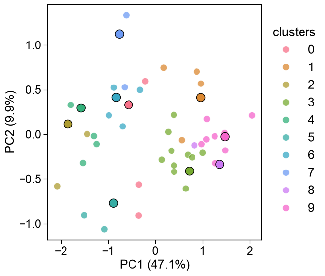
Visualizing the representative proteins

The protein clustering is visualized with the same AAclustPlot.medoids method, but here the input is the per-protein feature matrix X (samples × features), passed as-is: proteins need no transpose, unlike the df_scales form used for scales above. The method projects X into PCA space and marks the representative protein (medoid) of each cluster.

# Visualize the protein clusters and their representatives (medoids) in PCA space
aac_plot = aa.AAclustPlot()
aa.plot_settings()
fig, ax = aac_plot.medoids(X, labels=df_repr["cluster"])
plt.tight_layout()
plt.show()

Feature-space vs. sequence-identity redundancy

select_proteins reduces redundancy in CPP feature space (physicochemical similarity). A complementary tool, filter_seq (CD-HIT; requires the pro extra), reduces redundancy by sequence identity, keeping one representative per cluster of similar sequences. Both annotate the proteins with the same cluster / is_representative columns, so they compose, but they answer different questions.

# Sequence-identity redundancy reduction with CD-HIT (requires aaanalysis[pro])
df_cdhit = aa.filter_seq(df_seq, method="cd-hit", similarity_threshold=0.7)
n_cpp = int(df_repr["is_representative"].sum())
n_seq = int(df_cdhit["is_representative"].sum())
print(f"representatives by select_proteins (CPP feature space): {n_cpp} of {len(df_seq)}")
print(f"representatives by filter_seq    (sequence identity):   {n_seq} of {len(df_seq)}")
aa.display_df(df_cdhit, n_rows=10, show_shape=True)

representatives by select_proteins (CPP feature space): 10 of 50
representatives by filter_seq    (sequence identity):   50 of 50
DataFrame shape: (50, 4)

	entry	cluster	identity_with_rep	is_representative
1	Q9ERC8	0	100.000000	1
2	Q63155	1	100.000000	1
3	Q8VHS2	2	100.000000	1
4	P08069	3	100.000000	1
5	Q15303	4	100.000000	1
6	Q6ZRH7	5	100.000000	1
7	P16234	6	100.000000	1
8	D3ZZK3	7	100.000000	1
9	P54763	8	100.000000	1
10	O94985	9	100.000000	1

At a 70% identity threshold, CD-HIT finds these substrate sequences non-redundant and keeps all of them, while select_proteins still compresses them to 10 physicochemical representatives. The two tools are complementary, not interchangeable: use filter_seq to drop near-duplicate sequences before training, and select_proteins to pick a diverse, interpretable subset in feature space.

For further details, see our Feature Engineering API, AAontology Usage Principels, and AAclust Usage Principels.