CPP: Identification of physicochemical signatures

Comparative Physicochemical Profiling (CPP) is a sequence-based algorithm for interpretable feature engineering. It is the centerpiece of AAanalysis, introduced in [Breimann25].

The aim of the CPP algorithm is to identify a set of unique, non-redundant features that are most discriminant between the test and reference group of sequences. We call this feature set and its visual representation the physicochemical signature of the test group, which can be interpreted at group and sample level with single-residue resolution.

We will demonstrate this in three steps:

1. Feature Creation

2. Group Level CPP Analysis

3. Sample Level CPP Analysis

Feature Creation

To create an CPP object, you just need to provide a valid df_parts DataFrame:

import aaanalysis as aa
aa.options["verbose"] = False
aa.options["random_state"] = 42

# Load example dataset
df_seq = aa.load_dataset(name="DOM_GSEC")
labels = df_seq["label"].to_list()
sf = aa.SequenceFeature()

# Create Parts
df_parts = sf.get_df_parts(df_seq=df_seq)

# Create CPP object and run with default splits and scales
cpp = aa.CPP(df_parts=df_parts)

A non-redundant set of physicochemical features is obtained through the CPP.run() method:

# Run CPP algorithm to obtain 100 features (default)
df_feat = cpp.run(labels=labels, n_filter=100)
aa.display_df(df=df_feat, n_rows=8, show_shape=True)

/Users/stephanbreimann/Programming/1Packages/aaanalysis/.claude/worktrees/pr222-fresh/aaanalysis/feature_engineering/_backend/cpp_run.py:143: UserWarning: CPP is using the Python kernel fallback — the compiled Cython extension is not available in this install. Output is bit-exact with the Cython path but ~2x slower. Reinstall via pip install --force-reinstall aaanalysis to fetch a prebuilt wheel.
  warnings.warn(

DataFrame shape: (100, 13)

	feature	category	subcategory	scale_name	scale_description	abs_auc	abs_mean_dif	mean_dif	std_test	std_ref	p_val_mann_whitney	p_val_fdr_bh	positions
1	TMD_C_JMD_C-Seg...2,3)-QIAN880106	Conformation	α-helix	α-helix (middle)	Weights for alp...ejnowski, 1988)	0.387000	0.118000	0.118000	0.068000	0.080000	0.000000	0.000000	27,28,29,30,31,32,33
2	TMD_C_JMD_C-Pat...,14)-CRAJ730103	Conformation	β-turn	β-turn	Normalized freq...d et al., 1973)	0.377000	0.285000	-0.285000	0.164000	0.177000	0.000000	0.000000	27,31
3	TMD_C_JMD_C-Seg...6,9)-FAUJ880104	Shape	Side chain length	Steric parameter	STERIMOL length...e et al., 1988)	0.367000	0.263000	0.263000	0.161000	0.168000	0.000000	0.000000	32,33
4	TMD_C_JMD_C-Seg...6,9)-ONEK900101	Others	Unclassified (Others)	ΔG values in peptides	Delta G values ...-DeGrado, 1990)	0.366000	0.111000	0.111000	0.070000	0.114000	0.000000	0.000000	32,33
5	TMD_C_JMD_C-Pat...,15)-QIAN880107	Conformation	α-helix	α-helix (middle)	Weights for alp...ejnowski, 1988)	0.363000	0.162000	0.162000	0.091000	0.118000	0.000000	0.000000	24,28,32,35
6	TMD_C_JMD_C-Seg...3,4)-HUTJ700103	Energy	Entropy	Entropy	Entropy of form...Hutchens, 1970)	0.360000	0.187000	0.187000	0.115000	0.128000	0.000000	0.000000	31,32,33,34,35
7	TMD_C_JMD_C-Seg...2,3)-WOLS870103	Others	PC 4	Principal Component 3 (Wold)	Principal prope...d et al., 1987)	0.359000	0.159000	-0.159000	0.090000	0.130000	0.000000	0.000000	27,28,29,30,31,32,33
8	TMD_C_JMD_C-Pat...,12)-CRAJ730103	Conformation	β-turn	β-turn	Normalized freq...d et al., 1973)	0.352000	0.227000	-0.227000	0.150000	0.170000	0.000000	0.000000	24,28,32

CPP Analysis (Group Level)

The CPPPlot class provides various methods for visualizing single to all features. For further analysis, we need to add the group level feature importance using the TreeModel class:

# Create feature matrix
sf = aa.SequenceFeature()
X = sf.feature_matrix(features=df_feat["feature"], df_parts=df_parts)

# Fit TreeModel
tm = aa.TreeModel()
tm = tm.fit(X, labels=labels)

# Add feature importance, ranked most-important-first via sort=True
df_feat = tm.add_feat_importance(df_feat=df_feat, sort=True)

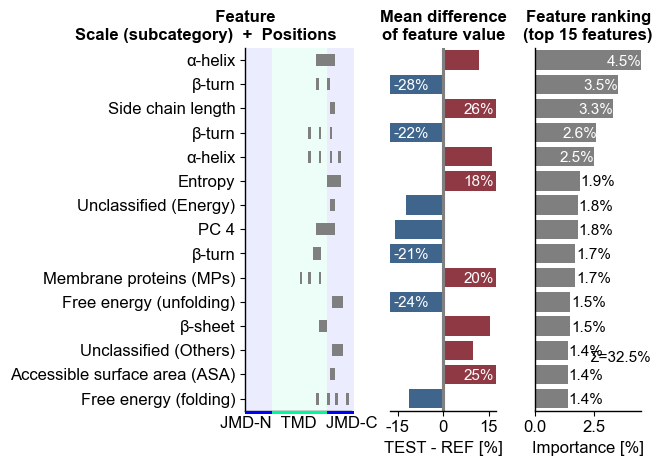
The top 15 features can be visualized using the CPPPlot.ranking() method

import matplotlib.pyplot as plt

# CPP ranking
cpp_plot = aa.CPPPlot()
aa.plot_settings(weight_bold=False, short_ticks=True)
cpp_plot.ranking(df_feat=df_feat)
plt.tight_layout()
plt.show()

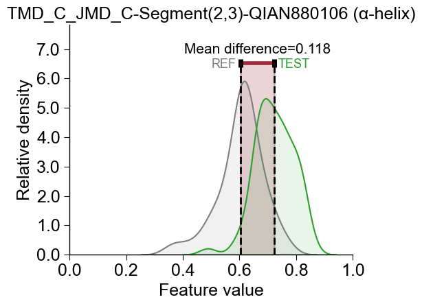
The difference of feature values between the test and the reference group can be displayed for any selected feature using the CPPPlot.feature() method:

# df_feat is already sorted by feat_importance (sort=True above), so feat_rank=1 is the top feature
# Show feature value distribution for the best feature
aa.plot_settings()
cpp_plot.feature(feature=df_feat, feat_rank=1, df_seq=df_seq, labels=labels)
plt.title(f"{df_feat['feature'][0]} ({df_feat['subcategory'][0]})")
plt.tight_layout()
plt.show()

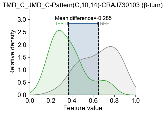
The feature value difference can be either positive (the test dataset has higher values, indicated in red) or negative (the test dataset has lower values, indicated in blue):

# feat_rank=2 selects the second-best feature from the ranked df_feat
aa.plot_settings()
cpp_plot.feature(feature=df_feat, feat_rank=2, df_seq=df_seq, labels=labels)
plt.title(f"{df_feat['feature'][1]} ({df_feat['subcategory'][1]})")
plt.tight_layout()
plt.show()

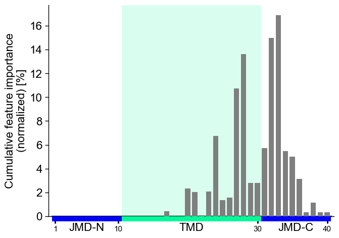
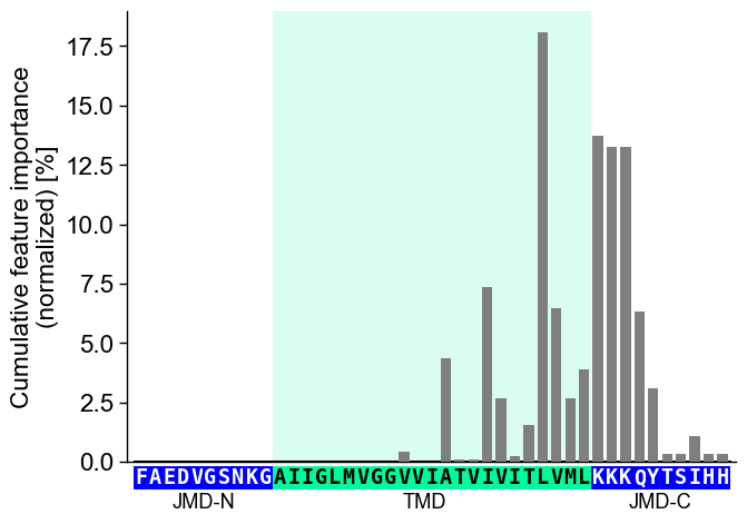
To visualize the importance of all features at single-residue resolution, the cumulative feature importance per residue position can be shown using the CPPPlot.profile() method:

# Plot CPP profile
aa.plot_settings(font_scale=0.9)
cpp_plot.profile(df_feat=df_feat)
plt.tight_layout()
plt.show()

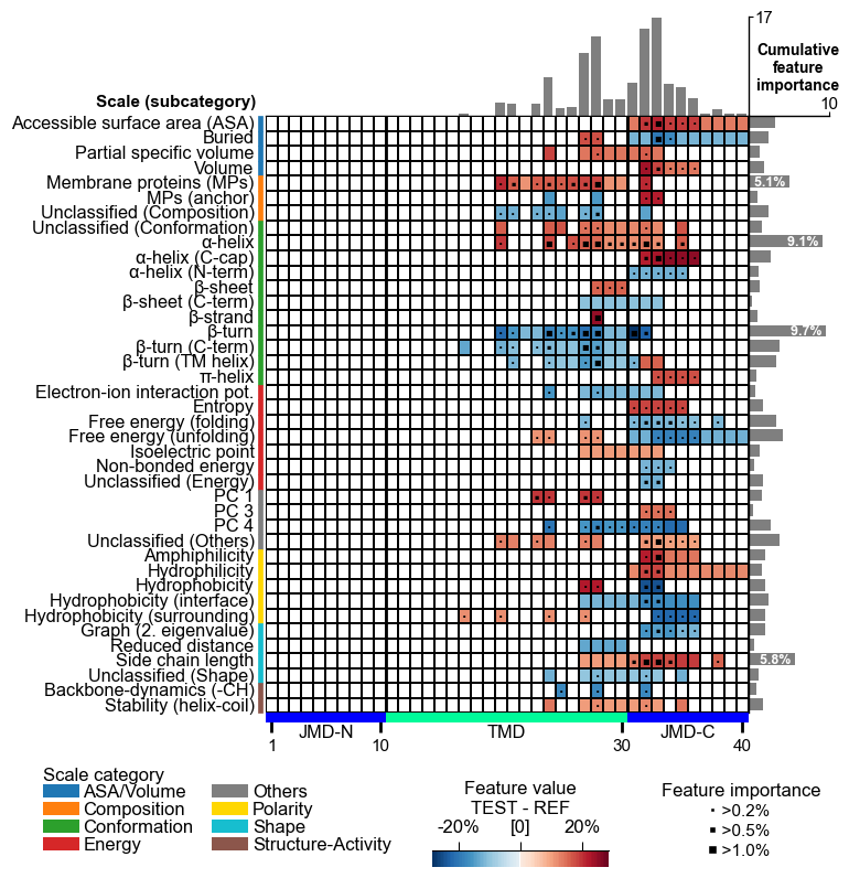
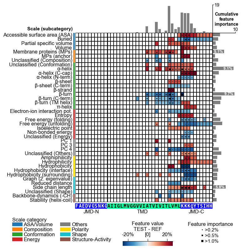
The complete feature landscape can be charted using the CPPPlot.feature_map() method. This CPP feature map shows the feature value difference and feature importance per residue and scale subcategory, which are described and discussed in our `AAontology`` (AAontology Usage Principles, [Breimann24b]):

# Plot CPP feature map
cpp_plot = aa.CPPPlot()
aa.plot_settings(font_scale=0.65, weight_bold=False)
cpp_plot.feature_map(df_feat=df_feat)
plt.show()

CPP Analysis (“Sample Level”)

You can provide individual sequence parts to the plotting methods to translate the results of the group level CPP features onto a specific sample.

# Get sequences parts for APP
seq_kws = sf.get_seq_kws(df_seq=df_seq, df_parts=df_parts, sample="P05067")

Provide the parts as tmd_seq, jmd_n_seq, and jmd_c_seq parameters to the CPPPlot.profile() method:

# Plot CPP profile ("sample level")
aa.plot_settings(font_scale=0.9)
cpp_plot.profile(df_feat=df_feat, **seq_kws)
plt.tight_layout()
plt.show()

Or to the CPPPlot.feature_map method:

# Plot CPP feature map ("sample level")
cpp_plot = aa.CPPPlot()
aa.plot_settings(font_scale=0.65, weight_bold=False)
cpp_plot.feature_map(df_feat=df_feat, **seq_kws)
plt.show()

However, these are still the general results but only visualized for a specific sample sequence. To obtain the sample-specific feature value difference and feature impact, see the Explainable AI Tutorial.

For more details on the CPP and CPPPlot classes are given in the Feature Engineering API. To delve deeper into the feature concept, see the CPP Usage Principles section.