A minimal CPP analysis
The shortest complete loop in AAanalysis: load a dataset, run Comparative Physicochemical Profiling (CPP) with its defaults, and read out the physicochemical signature that separates the two groups — first as a ranked list, then as a feature map.
We use the domain-level γ-secretase dataset (DOM_GSEC: substrates
vs. non-substrates) and lean on defaults throughout: CPP loads a default
amino-acid scale set for you, so there is nothing to select or tune. For
the broader tour (machine learning, SHAP feature impact, the comparison
harness) see the Quick start tutorial.
You will learn to use the tool below — its inputs, outputs, key parameters, and how to inspect the result.
Tool —
SequenceFeature,CPP,TreeModel,CPPPlotInput —
df_seq(sequences with a binarylabel)Output —
df_feat(the CPP signature) plus a feature mapBest used for — a four-step first taste of the load -> CPP -> signature loop before choosing the right setup for your own task
Related protocol — P1: CPP signature
Related API — :class:`~aaanalysis.CPP,
CPPPlot<https://aaanalysis.readthedocs.io/en/latest/api.html#feature-engineering>`__
import matplotlib.pyplot as plt

import aaanalysis as aa
aa.options["verbose"] = False
aa.options["random_state"] = 42
1. Load a dataset
load_dataset() returns a sequence table (df_seq) with the TMD
bounds. Its binary label column is the A-vs-B grouping that CPP
contrasts.
df_seq = aa.load_dataset(name="DOM_GSEC", n=50)
labels = df_seq["label"].to_list()
aa.display_df(df=df_seq, n_rows=10, show_shape=True)
DataFrame shape: (100, 8)
| entry | sequence | label | tmd_start | tmd_stop | jmd_n | tmd | jmd_c | |
|---|---|---|---|---|---|---|---|---|
| 1 | Q14802 | MQKVTLGLLVFLAGF...PGETPPLITPGSAQS | 0 | 37 | 59 | NSPFYYDWHS | LQVGGLICAGVLCAMGIIIVMSA | KCKCKFGQKS |
| 2 | Q86UE4 | MAARSWQDELAQQAE...SPKQIKKKKKARRET | 0 | 50 | 72 | LGLEPKRYPG | WVILVGTGALGLLLLFLLGYGWA | AACAGARKKR |
| 3 | Q969W9 | MHRLMGVNSTAAAAA...AIWSKEKDKQKGHPL | 0 | 41 | 63 | FQSMEITELE | FVQIIIIVVVMMVMVVVITCLLS | HYKLSARSFI |
| 4 | P53801 | MAPGVARGPTPYWRL...GLFKEENPYARFENN | 0 | 97 | 119 | RWGVCWVNFE | ALIITMSVVGGTLLLGIAICCCC | CCRRKRSRKP |
| 5 | Q8IUW5 | MAPRALPGSAVLAAA...EVPATPVKRERSGTE | 0 | 59 | 81 | NDTGNGHPEY | IAYALVPVFFIMGLFGVLICHLL | KKKGYRCTTE |
| 6 | P01135 | MVPSAGQLALFALGI...LLKGRTACCHSETVV | 0 | 99 | 121 | AVVAASQKKQ | AITALVVVSIVALAVLIITCVLI | HCCQVRKHCE |
| 7 | O43914 | MGGLEPCSRLLLLPL...SDVYSDLNTQRPYYK | 0 | 42 | 64 | DCSCSTVSPG | VLAGIVMGDLVLTVLIALAVYFL | GRLVPRGRGA |
| 8 | P05556 | MNLQPIFWIGLISSV...KSAVTTVVNPKYEGK | 0 | 729 | 751 | ENPECPTGPD | IIPIVAGVVAGIVLIGLALLLIW | KLLMIIHDRR |
| 9 | P16234 | MGTSHPAFLVLGCLL...DIGIDSSDLVEDSFL | 0 | 527 | 549 | VAPTLRSELT | VAAAVLVLLVIVIISLIVLVVIW | KQKPRYEIRW |
| 10 | P50895 | MEPPDAPAQARGAPR...SGGARGGSGGFGDEC | 0 | 549 | 571 | TVSPQTSQAG | VAVMAVAVSVGLLLLVVAVFYCV | RRKGGPCCRQ |
2. Run CPP
SequenceFeature builds the parts (the TMD and its juxtamembrane
flanks) that CPP profiles. CPP then creates all Part × Split ×
Scale features over a default scale set — no scale selection needed
— contrasts the two groups, and returns the ranked, non-redundant
feature table df_feat.
sf = aa.SequenceFeature()
df_parts = sf.get_df_parts(df_seq=df_seq)
cpp = aa.CPP(df_parts=df_parts)
df_feat = cpp.run(labels=labels)
aa.display_df(df=df_feat, n_rows=10, show_shape=True)
DataFrame shape: (100, 13)
| feature | category | subcategory | scale_name | scale_description | abs_auc | abs_mean_dif | mean_dif | std_test | std_ref | p_val_mann_whitney | p_val_fdr_bh | positions | |
|---|---|---|---|---|---|---|---|---|---|---|---|---|---|
| 1 | TMD_C_JMD_C-Seg...2,3)-QIAN880106 | Conformation | α-helix | α-helix (middle) | Weights for alp...ejnowski, 1988) | 0.387000 | 0.121000 | 0.121000 | 0.069000 | 0.085000 | 0.000000 | 0.000001 | 27,28,29,30,31,32,33 |
| 2 | TMD_C_JMD_C-Seg...5,7)-FAUJ880104 | Shape | Side chain length | Steric parameter | STERIMOL length...e et al., 1988) | 0.382000 | 0.264000 | 0.264000 | 0.156000 | 0.156000 | 0.000000 | 0.000001 | 32,33,34 |
| 3 | TMD_C_JMD_C-Pat...,12)-ROBB760109 | Conformation | β-turn (N-term) | β-turn (1st residue) | Information mea...n-Suzuki, 1976) | 0.377000 | 0.127000 | -0.127000 | 0.062000 | 0.088000 | 0.000000 | 0.000001 | 21,25,28,32 |
| 4 | TMD_C_JMD_C-Seg...4,5)-ZIMJ680104 | Energy | Isoelectric point | Isoelectric point | Isoelectric poi...n et al., 1968) | 0.373000 | 0.220000 | 0.220000 | 0.124000 | 0.137000 | 0.000000 | 0.000001 | 33,34,35,36 |
| 5 | TMD_C_JMD_C-Seg...5,7)-ONEK900101 | Others | Unclassified (Others) | ΔG values in peptides | Delta G values ...-DeGrado, 1990) | 0.373000 | 0.115000 | 0.115000 | 0.066000 | 0.113000 | 0.000000 | 0.000001 | 32,33,34 |
| 6 | TMD_C_JMD_C-Seg...4,5)-WOLS870103 | Others | PC 4 | Principal Component 3 (Wold) | Principal prope...d et al., 1987) | 0.370000 | 0.218000 | -0.218000 | 0.123000 | 0.169000 | 0.000000 | 0.000001 | 33,34,35,36 |
| 7 | TMD_C_JMD_C-Seg...2,3)-WOLS870103 | Others | PC 4 | Principal Component 3 (Wold) | Principal prope...d et al., 1987) | 0.365000 | 0.154000 | -0.154000 | 0.096000 | 0.123000 | 0.000000 | 0.000001 | 27,28,29,30,31,32,33 |
| 8 | TMD_C_JMD_C-Seg...4,5)-FINA910103 | Conformation | α-helix (C-cap) | α-helix (C-terminal, inside) | Helix terminati...n et al., 1991) | 0.362000 | 0.264000 | 0.264000 | 0.157000 | 0.175000 | 0.000000 | 0.000001 | 33,34,35,36 |
| 9 | TMD_C_JMD_C-Pat...,15)-QIAN880107 | Conformation | α-helix | α-helix (middle) | Weights for alp...ejnowski, 1988) | 0.359000 | 0.158000 | 0.158000 | 0.081000 | 0.122000 | 0.000000 | 0.000001 | 25,28,32,35 |
| 10 | TMD_C_JMD_C-Pat...,15)-MUNV940101 | Energy | Free energy (folding) | Free energy (α-helix) | Free energy in ...-Serrano, 1994) | 0.358000 | 0.097000 | -0.097000 | 0.050000 | 0.082000 | 0.000000 | 0.000001 | 24,28,32,35 |
3. Score feature importance
A TreeModel scores how much each feature helps tell the two groups
apart and writes that back as the feat_importance column that the
plots rank by.
X = sf.feature_matrix(df_feat, df_parts)
tm = aa.TreeModel()
tm.fit(X, labels=labels)
df_feat = tm.add_feat_importance(df_feat=df_feat)
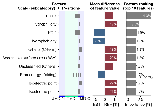
4. Read out the signature
ranking() lists the top features — each an interpretable,
residue-grounded Part × Split × Scale combination — which together
form the physicochemical signature of the substrates.
cpp_plot = aa.CPPPlot()
aa.plot_settings(short_ticks=True, weight_bold=False)
cpp_plot.ranking(df_feat=df_feat, n_top=10)
plt.tight_layout()
plt.show()
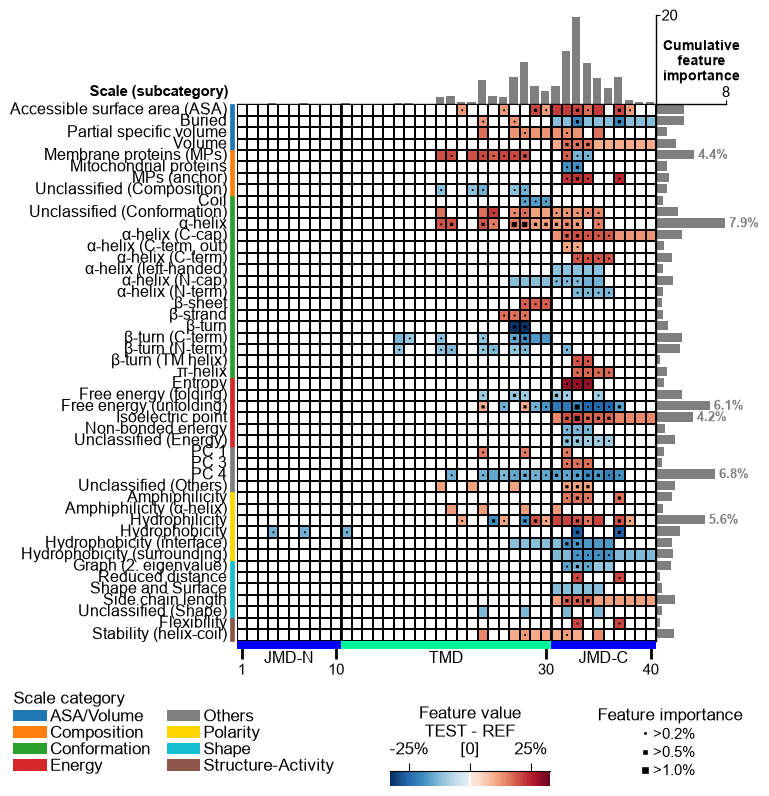
feature_map() then charts the whole signature in a single
figure — every selected Part × Split × Scale feature placed by scale
subcategory (y-axis) and residue position (x-axis), colored by the group
mean difference and marked by feature importance. It is the most
complete single-figure read-out of a CPP analysis.
aa.plot_settings(font_scale=0.65, weight_bold=False)
cpp_plot.feature_map(df_feat=df_feat)
plt.show()
That is the whole loop: data → CPP → signature. To pick the right setup for your task — residue, domain, or protein level — see the Prediction tasks page, and the Protocols for end-to-end workflows.