aaanalysis.CPPPlot.ranking

CPPPlot.ranking(df_feat=None, shap_plot=False, col_dif='mean_dif', col_imp='feat_importance', rank=True, n_top=15, figsize=(7, 5), tmd_len=20, tmd_jmd_space=2, tmd_color='mediumspringgreen', jmd_color='blue', tmd_jmd_alpha=0.075, name_test='TEST', name_ref='REF', fontsize_titles=12, fontsize_labels=12, fontsize_annotations=11, xlim_dif=(-17.5, 17.5), xlim_rank=(0, 4), rank_info_xy=None)

Plot CPP/-SHAP feature ranking based on feature importance or sample-specif feature impact.

Introduced in [Breimann25a], this method visualizes the most important features for discriminating between the test and the reference dataset groups. At sample level, the feature impact derived from SHAP values of a specific sample can be used for ranking if shap_plot=True and ‘feature_impact’ column in df_feat.

Parameters:

• df_feat (pd.DataFrame, shape (n_features, n_feature_info)) – Feature DataFrame with a unique identifier, scale information, statistics, and positions for each feature. Must also include feature importance (feat_importance) or impact (feat_impact_'name') columns.

• shap_plot (bool, default=False) –

  Set the analysis type: CPP Analysis (if False) for group-level or CPP-SHAP Analysis for sample-level (or subgroup-level) results:

  CPP Analysis

  • col_dif: Displays the group-level difference of feature values, with the mean_dif column selected by default.

  • col_imp: Refers to the group-level feat_importance column (shown in gray) used for feature ranking.

  CPP-SHAP Analysis

  • col_dif: Allows the selection of sample-specific differences against the reference group from a mean_dif_’name’ column.

  • col_imp: Enables the selection of specific feature impacts from a feat_impact_’name’ column for an individual sample, where positive (red) and negative (blue) feature impacts are visualized in the ranking.

• col_dif (str, default='mean_dif') – Column name in df_feat for differences in feature values. Must match with the shap_plot setting.

• col_imp (str, default='feat_importance') – Column name in df_feat for feature importance/impact values. Must match with the shap_plot setting.

• rank (bool, default=True) – If True, features will be ranked in descending order of col_imp values.

• n_top (int, default=15) – The number of top features to display. Should be 1 < n_top <= n_features.

• figsize (tuple, default=(7, 5)) – Figure dimensions (width, height) in inches.

• tmd_len (int, default=20) – Length of TMD to be depicted (>0).

• tmd_jmd_space (int, default=2) – The space between TMD and JMD labels (>0) in the feature position subplot.

• tmd_color (str, default='mediumspringgreen') – Color for TMD.

• jmd_color (str, default='blue') – Color for JMDs.

• tmd_jmd_alpha (int or float, default=0.075) – The transparency alpha value [0-1] of the TMD-JMD area in the feature position subplot.

• name_test (str, default="TEST") – Name of the test dataset to show in the mean difference subplot.

• name_ref (str, default="REF") – Name of reference dataset to show in the mean difference subplot.

• fontsize_titles (int or float, default=12) – Font size of the titles.

• fontsize_labels (int or float , default=12) – Font size of plot labels.

• fontsize_annotations (int or float, default=11) – Font size of annotations.

• xlim_dif (tuple, default=(-17.5, 17.5)) – x-axis limits for the mean difference subplot.

• xlim_rank (tuple, default=(0, 4)) – x-axis limits for the ranking subplot. If None, determined automatically.

• rank_info_xy (tuple, optional) –

  Position (x-axis, y-axis) in ranking subplot for showing additional information (optimized if None):

  • When shap_plot=False: Displays sum of feature importance.

  • When shap_plot=True: Show the sum of the absolute feature impact and the SHAP legend.

Returns:

• fig (plt.Figure) – The Figure object for the ranking plot.

• axes (array of plt.Axes) – Array of Axes objects, each representing a subplot within the figure.

Notes

• Features are shown as ordered in df_feat. A ranking in descending order based one the following columns is recommended:

  • feat_importance: when feature importance is in df_feat and shap_plot=False.

  • feat_impact_'name': when sample-specific feature impact is in df_feat and shap_plot=True.

See also

• CPP.run() for details on CPP statistical measures of the df_feat DataFrame.

• SequenceFeature for definition of sequence Parts.

• CPPPlot.feature() for visualization of mean differences for specific features.

Examples

To demonstrate the CPPPlot().ranking() method, we first load the example feature set from for the DOM_GSEC data (see [Breimann25a]):

import matplotlib.pyplot as plt
import aaanalysis as aa
aa.options["verbose"] = False

df_feat = aa.load_features()
df_feat = df_feat.sort_values(by="feat_importance", ascending=False).reset_index(drop=True)
aa.display_df(df_feat, show_shape=True, n_rows=20)

DataFrame shape: (150, 15)

	feature	category	subcategory	scale_name	scale_description	abs_auc	abs_mean_dif	mean_dif	std_test	std_ref	p_val_mann_whitney	p_val_fdr_bh	positions	feat_importance	feat_importance_std
1	TMD_C_JMD_C-Seg...,11)-LIFS790102	Conformation	β-strand	β-strand	Conformational ...n-Sander, 1979)	0.189000	0.125674	0.125674	0.183876	0.218813	0.000001	0.000039	28,29	4.729200	4.776785
2	TMD_C_JMD_C-Seg...2,3)-CHOP780212	Conformation	β-sheet (C-term)	β-turn (1st residue)	Frequency of th...-Fasman, 1978b)	0.199000	0.065983	-0.065983	0.087814	0.105835	0.000000	0.000016	27,28,29,30,31,32,33	4.106000	5.236574
3	TMD_C_JMD_C-Seg...3,4)-HUTJ700102	Energy	Entropy	Entropy	Absolute entrop...Hutchens, 1970)	0.229000	0.098224	0.098224	0.106865	0.124608	0.000000	0.000001	31,32,33,34,35	3.111200	3.109955
4	TMD_C_JMD_C-Seg...2,3)-AURR980110	Conformation	α-helix	α-helix (middle)	Normalized posi...ora-Rose, 1998)	0.211000	0.077355	0.077355	0.102965	0.107453	0.000000	0.000005	27,28,29,30,31,32,33	3.048800	3.623912
5	TMD_C_JMD_C-Pat...4,8)-JANJ790102	Energy	Free energy (unfolding)	Transfer free e...(TFE) to inside	Transfer free e...y (Janin, 1979)	0.187000	0.144354	-0.144354	0.181777	0.233103	0.000001	0.000049	33,37	2.833600	3.640617
6	TMD_C_JMD_C-Pat...4,8)-KANM800103	Conformation	α-helix	α-helix	Average relativ...sa-Tsong, 1980)	0.176000	0.087846	0.087846	0.140464	0.157561	0.000004	0.000113	24,28	2.704000	4.076269
7	TMD_C_JMD_C-Pat...,10)-LEVM760105	Shape	Side chain length	Side chain length	Radius of gyrat... (Levitt, 1976)	0.149000	0.073526	0.073526	0.133612	0.157088	0.000090	0.000714	31,34,38	2.050800	2.338278
8	TMD_C_JMD_C-Seg...4,5)-LEVM760105	Shape	Side chain length	Side chain length	Radius of gyrat... (Levitt, 1976)	0.204000	0.105513	0.105513	0.132849	0.145219	0.000000	0.000009	33,34,35,36	1.992000	2.929460
9	TMD_C_JMD_C-Seg...,11)-QIAN880134	Conformation	Coil	Coil	Weights for coi...ejnowski, 1988)	0.181000	0.057287	-0.057287	0.072234	0.106512	0.000002	0.000076	28,29	1.919600	2.094497
10	TMD-PeriodicPat...3,4)-VELV850101	Energy	Electron-ion interaction pot.	Electron-ion in...ction potential	Electron-ion in...c et al., 1985)	0.180000	0.069277	-0.069277	0.094949	0.119524	0.000002	0.000082	13,16,20,23,27	1.818000	2.308293
11	TMD_C_JMD_C-Seg...6,9)-AURR980110	Conformation	α-helix	α-helix (middle)	Normalized posi...ora-Rose, 1998)	0.211000	0.125350	0.125350	0.160819	0.174121	0.000000	0.000005	32,33	1.788800	2.700803
12	TMD_C_JMD_C-Seg...,10)-WILM950103	Polarity	Hydrophobicity (interface)	Hydrophobicity (interface)	Hydrophobicity ...e et al., 1995)	0.212000	0.141305	-0.141305	0.168603	0.217235	0.000000	0.000005	33,34	1.747200	2.150664
13	TMD_C_JMD_C-Seg...,11)-COHE430101	ASA/Volume	Partial specific volume	Partial specific volume	Partial specifi...n-Edsall, 1943)	0.145000	0.124999	0.124999	0.180151	0.242281	0.000145	0.000912	28,29	1.740800	2.317117
14	TMD_C_JMD_C-Pat...5,8)-RADA880104	Energy	Free energy (unfolding)	Transfer free e...(TFE) to inside	Transfer free e...olfenden, 1988)	0.197000	0.060758	0.060758	0.050818	0.095267	0.000000	0.000019	25,28	1.658800	3.421774
15	JMD_N_TMD_N-Seg...1,2)-KARP850101	Structure-Activity	Flexibility	Flexibility (0 ...igid neighbors)	Flexibility par...s-Schulz, 1985)	0.196000	0.062671	0.062671	0.083456	0.090427	0.000000	0.000023	1,2,3,4,5,6,7,8,9,10	1.574400	1.835403
16	TMD_C_JMD_C-Seg...6,9)-LEVM760105	Shape	Side chain length	Side chain length	Radius of gyrat... (Levitt, 1976)	0.233000	0.137044	0.137044	0.161683	0.176964	0.000000	0.000001	32,33	1.554800	2.109848
17	TMD_C_JMD_C-Pat...5,8)-QIAN880130	Conformation	Coil	Coil	Weights for coi...ejnowski, 1988)	0.162000	0.070292	-0.070292	0.096915	0.128362	0.000020	0.000302	21,25,28	1.528400	2.418922
18	TMD-Pattern(C,5...,15)-OOBM770105	Energy	Non-bonded energy	Non-bonded energy per residue	Short and mediu...take-Ooi, 1977)	0.164000	0.056983	0.056983	0.099221	0.102039	0.000017	0.000274	16,19,22,26	1.305600	1.643621
19	JMD_N_TMD_N-Pat...,11)-PRAM820103	Shape	Shape and Surface	Correlation coe...t in regression	Correlation coe...nnuswamy, 1982)	0.161000	0.057828	0.057828	0.088362	0.106085	0.000024	0.000328	1,5,8,11	1.304400	1.657101
20	TMD-Pattern(C,4,7)-VELV850101	Energy	Electron-ion interaction pot.	Electron-ion in...ction potential	Electron-ion in...c et al., 1985)	0.165000	0.121210	-0.121210	0.143560	0.207767	0.000015	0.000254	24,27	1.302000	1.466618

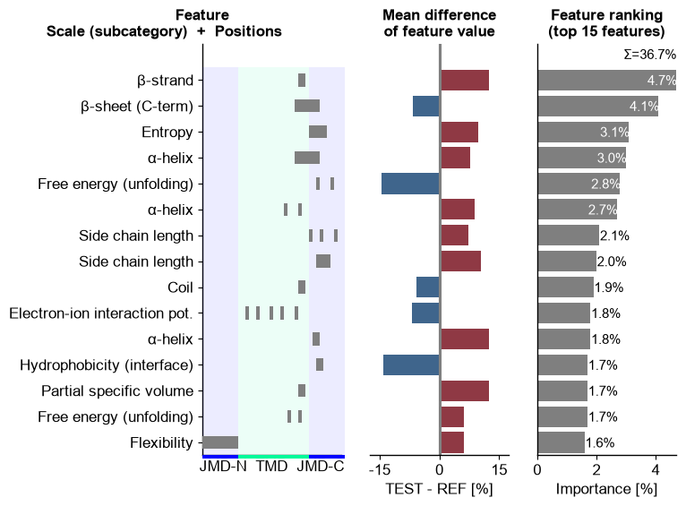
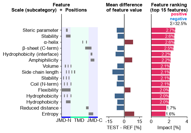
You can now create the CPP-Ranking Plot, which shows the features in the order of the df_feat DataFrame. Three subplots are given (from left to right):

1. Feature Position Subplot: Shows the position of the respective Part-Split combinations depending on the size of the TMD and JMDs.

2. Feature Mean Difference Subplot: Shows the mean differences between the test and reference dataset. Higher values for the test set are indicated in red and lower values in blue.

3. Feature Ranking Subplot: Shows the feature importance (or sample-specific impact) as bar chart.

cpp_plot = aa.CPPPlot()
aa.plot_settings(weight_bold=False, short_ticks=True)
cpp_plot.ranking(df_feat=df_feat)
plt.tight_layout()
plt.show()

Select the number of features using the n_top parameter:

# Show ranking of top 20 features
cpp_plot.ranking(df_feat=df_feat, n_top=20)
plt.tight_layout()
plt.show()

Disable the sorting in descending of feature importance order by setting rank=False (default=True):

# Show 15 random features
cpp_plot.ranking(df_feat=df_feat.sample(15), rank=False)
plt.tight_layout()
plt.show()

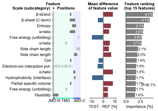
You can adjust the TMD size using the tmd_len parameter and the sizes of the JMDs using the jmd_c_len and jmd_n_len attributes of the CPPPlot class:

# Change part length
cpp_plot = aa.CPPPlot(jmd_n_len=5, jmd_c_len=20)
cpp_plot.ranking(df_feat=df_feat, tmd_len=50)
plt.tight_layout()
plt.show()

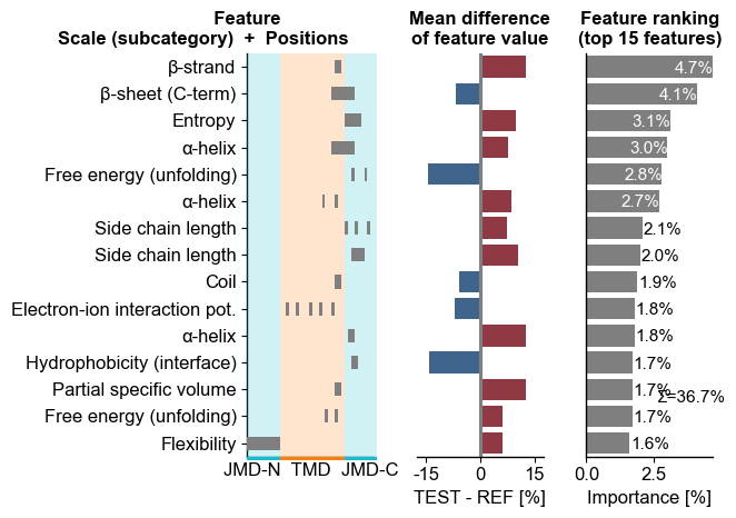
Adjust the colors and transparency using the tmd_color, jmd_color, and tmd_jmd_alpha parameters:

# Create a new CPPPlot object with default jmd length
cpp_plot = aa.CPPPlot()
cpp_plot.ranking(df_feat=df_feat, tmd_color="tab:orange", jmd_color="tab:cyan", tmd_jmd_alpha=0.2)
plt.tight_layout()
plt.show()

For the Feature Mean Difference Subplot, you can adjust the name of the test and reference dataset using the name_test and name_ref parameters:

# Change name of datasets
cpp_plot.ranking(df_feat=df_feat, name_test="Test set", name_ref="Reference set")
plt.tight_layout()
plt.show()

Potential overlap of labels and other fonts can be mitigated by adjusting the font sizes using the following parameters: fontsize_titles (default=10), fontsize_labels (default=11), and fontsize_annotations (default=11):

# Adjust font sizes
cpp_plot.ranking(df_feat=df_feat,
                 name_test="Test set", name_ref="Reference set",
                 fontsize_titles=13, fontsize_labels=8, fontsize_annotations=12)
plt.tight_layout()
plt.show()

Increase the distance of TMD and JMD labels using the tmd_jmd_space (default=2) parameter:

# Change spacing between TMD and JMDs
cpp_plot.ranking(df_feat=df_feat,
                 name_test="Test set", name_ref="Reference set",
                 tmd_jmd_space=6)
plt.tight_layout()
plt.show()

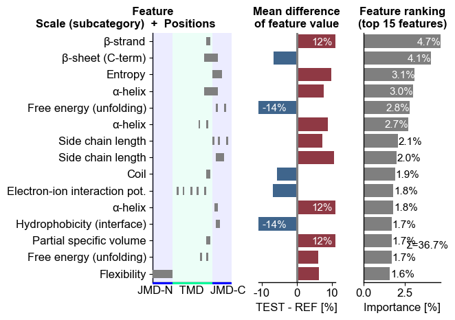
You can adjust the x-limits using xlim_dif and xlim_rank. Mean difference values exceeding the set x-axis limit are given on the respective bars:

# Modify x-axis limits
cpp_plot.ranking(df_feat=df_feat, xlim_dif=(-11, 11), xlim_rank=(0, 4))
plt.tight_layout()
plt.show()

To avoid an overlap of bars with the ranking information (the total feature importance if shap_plot=False), you can change its x-axis and y-axis position using the rank_info_xy parameter:

cpp_plot.ranking(df_feat=df_feat, xlim_dif=(-11, 11), xlim_rank=(0, 4), rank_info_xy=(4, 13))
plt.tight_layout()
plt.show()

CPP-SHAP analysis

Set shap_plot=True for visualizing the sample-specific feature impact instead of the overall feature importance. To demonstrate this we first obtain the DOM_GSEC example dataset, matching to the already used feature set (see [Breimann25a]):

aa.options["verbose"] = False
# Load example dataset
df_seq = aa.load_dataset(name="DOM_GSEC", n=3)
labels = df_seq["label"].to_list()

# Create feature matrix
sf = aa.SequenceFeature()
df_parts = sf.get_df_parts(df_seq=df_seq)
X = sf.feature_matrix(features=df_feat["feature"], df_parts=df_parts)

aa.display_df(df_seq)

	entry	sequence	label	tmd_start	tmd_stop	jmd_n	tmd	jmd_c
1	Q14802	MQKVTLGLLVFLAGF...PGETPPLITPGSAQS	0	37	59	NSPFYYDWHS	LQVGGLICAGVLCAMGIIIVMSA	KCKCKFGQKS
2	Q86UE4	MAARSWQDELAQQAE...SPKQIKKKKKARRET	0	50	72	LGLEPKRYPG	WVILVGTGALGLLLLFLLGYGWA	AACAGARKKR
3	Q969W9	MHRLMGVNSTAAAAA...AIWSKEKDKQKGHPL	0	41	63	FQSMEITELE	FVQIIIIVVVMMVMVVVITCLLS	HYKLSARSFI
4	P05067	MLPGLALLLLAAWTA...GYENPTYKFFEQMQN	1	701	723	FAEDVGSNKG	AIIGLMVGGVVIATVIVITLVML	KKKQYTSIHH
5	P14925	MAGRARSGLLLLLLG...EEEYSAPLPKPAPSS	1	868	890	KLSTEPGSGV	SVVLITTLLVIPVLVLLAIVMFI	RWKKSRAFGD
6	P70180	MRSLLLFTFSACVLL...RELREDSIRSHFSVA	1	477	499	PCKSSGGLEE	SAVTGIVVGALLGAGLLMAFYFF	RKKYRITIER

We can now include the feature impact into the df_feat for all samples using the ShapModel model:

sm = aa.ShapModel()
sm.fit(X, labels=labels)

# Include feature value difference for all samples against negatives
df_feat = sm.add_sample_mean_dif(X, labels=labels, df_feat=df_feat, drop=True)

# Include feature impact of all samples
df_feat = sm.add_feat_impact(df_feat=df_feat, drop=True)

aa.display_df(df_feat, n_rows=5)

	feature	category	subcategory	scale_name	scale_description	abs_auc	abs_mean_dif	mean_dif	std_test	std_ref	p_val_mann_whitney	p_val_fdr_bh	positions	mean_dif_Protein0	mean_dif_Protein1	mean_dif_Protein2	mean_dif_Protein3	mean_dif_Protein4	mean_dif_Protein5	feat_impact_Protein0	feat_impact_Protein1	feat_impact_Protein2	feat_impact_Protein3	feat_impact_Protein4	feat_impact_Protein5
1	TMD_C_JMD_C-Seg...,11)-LIFS790102	Conformation	β-strand	β-strand	Conformational ...n-Sander, 1979)	0.189000	0.125674	0.125674	0.183876	0.218813	0.000001	0.000039	28,29	0.286667	-0.192333	-0.094333	0.271667	0.286667	-0.083833	0.000000	0.000000	0.000000	0.000000	0.000000	0.000000
2	TMD_C_JMD_C-Seg...2,3)-CHOP780212	Conformation	β-sheet (C-term)	β-turn (1st residue)	Frequency of th...-Fasman, 1978b)	0.199000	0.065983	-0.065983	0.087814	0.105835	0.000000	0.000016	27,28,29,30,31,32,33	-0.048430	-0.023140	0.071570	-0.232290	-0.211860	-0.205570	-2.380000	-2.340000	-2.410000	2.040000	2.160000	2.030000
3	TMD_C_JMD_C-Seg...3,4)-HUTJ700102	Energy	Entropy	Entropy	Absolute entrop...Hutchens, 1970)	0.229000	0.098224	0.098224	0.106865	0.124608	0.000000	0.000001	31,32,33,34,35	0.131267	-0.269733	0.138467	0.231467	0.312467	0.277867	-0.710000	-0.700000	-0.720000	0.640000	0.960000	0.710000
4	TMD_C_JMD_C-Seg...2,3)-AURR980110	Conformation	α-helix	α-helix (middle)	Normalized posi...ora-Rose, 1998)	0.211000	0.077355	0.077355	0.102965	0.107453	0.000000	0.000005	27,28,29,30,31,32,33	0.036667	0.028807	-0.065473	0.137237	0.054097	0.041237	-0.430000	-0.420000	-0.430000	0.550000	0.560000	0.260000
5	TMD_C_JMD_C-Pat...4,8)-JANJ790102	Energy	Free energy (unfolding)	Transfer free e...(TFE) to inside	Transfer free e...y (Janin, 1979)	0.187000	0.144354	-0.144354	0.181777	0.233103	0.000001	0.000049	33,37	0.043333	0.228333	-0.271667	-0.030667	0.043333	-0.049167	0.020000	-0.130000	0.020000	0.040000	0.050000	0.040000

Finally, we can visualize the feature impact for a selected sample by providing the respective column name in col_imp and setting shap_plot=True:

# Show feature impact based on 6 samples
cpp_plot.ranking(df_feat=df_feat, col_imp="feat_impact_Protein4", shap_plot=True)
plt.tight_layout()
plt.show()

Sort the df_feat according the respective feature impact in descending order to show the top n features. We can further specify the feature value difference and the name for the specific sample using the col_dif and name_test parameters:

# Sort features in descending order for respective sample
df_feat = df_feat.sort_values(by="feat_impact_Protein4", ascending=False)

# Show ranked feature impact and feature value difference of Protein4 against negative samples
cpp_plot.ranking(df_feat=df_feat, col_dif="mean_dif_Protein4", col_imp="feat_impact_Protein4", name_test="Protein4", shap_plot=True)
plt.tight_layout()
plt.show()