P1: CPP signature
The key AAanalysis protocol. This workflow finds the physicochemical differences between two protein sets. Given two labelled sets of protein sequences (e.g. substrates vs. non-substrates, binders vs. non-binders, toxic vs. non-toxic), Comparative Physicochemical Profiling (CPP) identifies the set of position-resolved physicochemical features that most distinctly separate them, a determinant-discovery task that needs no black-box model. We call this feature set the signature of the test group.
CPP contrasts a test group (label=1) against a reference
group (label=0) and reads out what physicochemically
distinguishes them, and where. Behind the scenes it splits each
sequence into parts, applies splits (position selectors) within
each part, averages an amino-acid scale over those positions, and
keeps the Part-Split-Scale features that separate the two groups
best. The result is interpretable biology (an AAontology-grounded
signature), not a black box you have to trust on faith.
When to use it. Use this protocol when you have two labelled sets
of sequences and want to answer: “Which physicochemical patterns
distinguish my groups, and where in the sequence do they act?”, without
first committing to a black-box model. In glossary terms this is
determinant discovery: contrast a test group (label=1)
against a reference group (label=0) and read out what
physicochemically distinguishes them.
Typical questions: substrate vs. non-substrate, cleaved vs. not cleaved, aggregation-prone vs. soluble, toxic vs. non-toxic.
Here we work at the domain level (dataset prefix DOM_): the unit
of comparison is the transmembrane-domain (TMD) part set, native
ground for CPP.
When not to use it. CPP needs two labelled groups to contrast. If
you have no labels and just want to explore one set of sequences, start
with Protocol 0: Exploratory sequence analysis instead. If you already
trust a classifier and only want to know why it called this one protein
positive, that is a per-sample explanation task (see Protocol 8:
Interpretability, ShapModel). And CPP profiles part segments,
not long-range residue-residue contacts or inter-chain interfaces; those
are a documented scope boundary and belong to structure / PLM tooling.
Input. A df_seq with one row per protein and a binary label
column (test class = 1 vs. reference class = 0). For a domain-level
task it also carries tmd_start / tmd_stop (1-based, start- and
stop-inclusive), from which CPP derives the TMD-centric parts
jmd_n / tmd / jmd_c. This default part vocabulary fits a
domain-level task where the unit is a TMD; for another domain you
would rename the central tmd part to the specific domain name
(e.g. its Pfam/InterPro domain).
Here we use the bundled DOM_GSEC gamma-secretase dataset. The bridge
from sequences to CPP is get_df_parts(), which turns
df_seq into the df_parts that CPP consumes.
For a residue/window task you would construct windows first (see
Protocol 3: Construct sets & sampling); for embeddings/structure see
Protocol 4: Engineer features (run_num()).
import aaanalysis as aa

aa.options["verbose"] = False
aa.options["random_state"] = 42

# Two labelled sets of sequences (label: 1 = substrate/test, 0 = reference)
df_seq = aa.load_dataset(name="DOM_GSEC", n=50)
labels = df_seq["label"].to_list()
aa.display_df(df=df_seq, n_rows=5)
| entry | gene | sequence | label | tmd_start | tmd_stop | jmd_n | tmd | jmd_c | |
|---|---|---|---|---|---|---|---|---|---|
| 1 | Q14802 | FXYD3 | MQKVTLGLLVFLAGF...PGETPPLITPGSAQS | 0 | 37 | 59 | NSPFYYDWHS | LQVGGLICAGVLCAMGIIIVMSA | KCKCKFGQKS |
| 2 | Q86UE4 | MTDH | MAARSWQDELAQQAE...SPKQIKKKKKARRET | 0 | 50 | 72 | LGLEPKRYPG | WVILVGTGALGLLLLFLLGYGWA | AACAGARKKR |
| 3 | Q969W9 | PMEPA1 | MHRLMGVNSTAAAAA...AIWSKEKDKQKGHPL | 0 | 41 | 63 | FQSMEITELE | FVQIIIIVVVMMVMVVVITCLLS | HYKLSARSFI |
| 4 | P53801 | PTTG1IP | MAPGVARGPTPYWRL...GLFKEENPYARFENN | 0 | 97 | 119 | RWGVCWVNFE | ALIITMSVVGGTLLLGIAICCCC | CCRRKRSRKP |
| 5 | Q8IUW5 | RELL1 | MAPRALPGSAVLAAA...EVPATPVKRERSGTE | 0 | 59 | 81 | NDTGNGHPEY | IAYALVPVFFIMGLFGVLICHLL | KKKGYRCTTE |
Run. The real minimal path (not a one-liner): build sequence
parts with SequenceFeature, construct CPP on those parts and
call run with the labels, then rank the resulting signature by
importance with a TreeModel. CPP() takes df_parts, it does
not take df_seq/labels directly. (See the CPP tutorial
tutorial3c_cpp for the function details and parameters.) CPP is a
two-step method: run creates and coarse-filters the features,
then simplify refines them into a readable signature (shown next).
# 1) Split each sequence into parts (TMD / JMD-N / JMD-C by default)
sf = aa.SequenceFeature()
df_parts = sf.get_df_parts(df_seq=df_seq)

# 2) Run CPP on the parts to obtain the most discriminant features
#    (n_jobs=1 keeps it serial; multiprocessing spawn is fragile on
#    Python 3.14 + macOS without a __main__ guard)
cpp = aa.CPP(df_parts=df_parts)
df_feat_run = cpp.run(labels=labels, n_filter=50, n_jobs=1)
aa.display_df(df=df_feat_run, n_rows=8, show_shape=True)
DataFrame shape: (50, 13)
| feature | category | subcategory | scale_name | scale_description | abs_auc | abs_mean_dif | mean_dif | std_test | std_ref | p_val_mann_whitney | p_val_fdr_bh | positions | |
|---|---|---|---|---|---|---|---|---|---|---|---|---|---|
| 1 | TMD_C_JMD_C-Seg...2,3)-QIAN880106 | Conformation | α-helix | α-helix (middle) | Weights for alp...ejnowski, 1988) | 0.387000 | 0.121000 | 0.121000 | 0.069000 | 0.085000 | 0.000000 | 0.000000 | 27,28,29,30,31,32,33 |
| 2 | TMD_C_JMD_C-Seg...5,7)-FAUJ880104 | Shape | Side chain length | Steric parameter | STERIMOL length...e et al., 1988) | 0.382000 | 0.264000 | 0.264000 | 0.156000 | 0.156000 | 0.000000 | 0.000000 | 32,33,34 |
| 3 | TMD_C_JMD_C-Pat...,12)-ROBB760109 | Conformation | β-turn (N-term) | β-turn (1st residue) | Information mea...n-Suzuki, 1976) | 0.377000 | 0.127000 | -0.127000 | 0.062000 | 0.088000 | 0.000000 | 0.000000 | 21,25,28,32 |
| 4 | TMD_C_JMD_C-Seg...4,5)-ZIMJ680104 | Energy | Isoelectric point | Isoelectric point | Isoelectric poi...n et al., 1968) | 0.373000 | 0.220000 | 0.220000 | 0.124000 | 0.137000 | 0.000000 | 0.000000 | 33,34,35,36 |
| 5 | TMD_C_JMD_C-Seg...5,7)-ONEK900101 | Others | Unclassified (Others) | ΔG values in peptides | Delta G values ...-DeGrado, 1990) | 0.373000 | 0.115000 | 0.115000 | 0.066000 | 0.113000 | 0.000000 | 0.000000 | 32,33,34 |
| 6 | TMD_C_JMD_C-Seg...4,5)-WOLS870103 | Others | PC 4 | Principal Component 3 (Wold) | Principal prope...d et al., 1987) | 0.370000 | 0.218000 | -0.218000 | 0.123000 | 0.169000 | 0.000000 | 0.000000 | 33,34,35,36 |
| 7 | TMD_C_JMD_C-Seg...2,3)-WOLS870103 | Others | PC 4 | Principal Component 3 (Wold) | Principal prope...d et al., 1987) | 0.365000 | 0.154000 | -0.154000 | 0.096000 | 0.123000 | 0.000000 | 0.000000 | 27,28,29,30,31,32,33 |
| 8 | TMD_C_JMD_C-Seg...4,5)-FINA910103 | Conformation | α-helix (C-cap) | α-helix (C-terminal, inside) | Helix terminati...n et al., 1991) | 0.362000 | 0.264000 | 0.264000 | 0.157000 | 0.175000 | 0.000000 | 0.000001 | 33,34,35,36 |
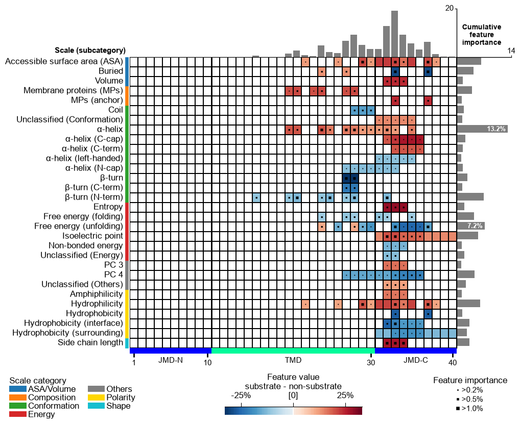
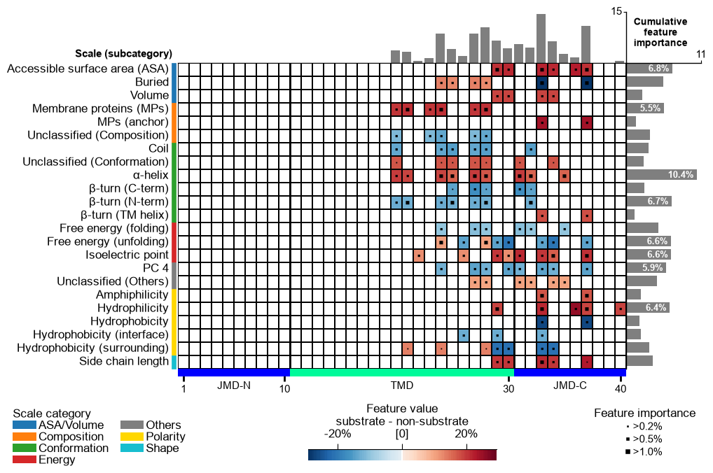
Look before you refine. The feature map is the lens for every step
below, so draw it first on the raw signature that run produced.
feature_map sizes its bars from a feat_importance column, so the
signature has to be ranked before it can be drawn: fit a TreeModel
on the CPP feature matrix and add the Monte-Carlo importance (percent).
Read the map as: rows = scale subcategories, columns = positions along the parts, colour = ``mean_dif`` (direction and strength), top bars = cumulative feature importance.
import matplotlib.pyplot as plt

# Rank the raw signature: a tree on the CPP feature matrix gives each feature a
# Monte-Carlo importance (percent), the column feature_map needs for its bars.
# add_feat_importance returns a NEW frame, so keep the ranked copy under its own
# name and leave df_feat_run as the plain run() output that simplify() consumes.
X_run = sf.feature_matrix(features=df_feat_run["feature"], df_parts=df_parts)
tm = aa.TreeModel()
tm = tm.fit(X_run, labels=labels)
df_run_ranked = tm.add_feat_importance(df_feat=df_feat_run)

# MAP 1 -- the raw signature: every Part-Split-Scale feature that run() kept.
aa.plot_settings(font_scale=0.6, weight_bold=False)
cpp_plot = aa.CPPPlot()
cpp_plot.feature_map(df_feat=df_run_ranked, name_test="substrate", name_ref="non-substrate")
plt.tight_layout()
plt.show()
Refine — the second CPP step: ``simplify``. CPP is a two-step
filter, and stopping after run is the most common reason a signature
reads as noise. run (above) creates and coarse-filters the raw
Part-Split-Scale features; simplify() then refines them
into a compact, more interpretable signature. For each feature it swaps
the scale for a correlated one from a better-graded AAontology
subcategory (interpretability grade 1-10, where 1 is best),
re-checks the swapped feature against the CPP filters and a
cross-validation gate (ml_model/ml_cv), and finally removes
redundancy — without ever dropping an original feature (only a
swapped feature that became redundant is removed). The result says the
same thing in fewer, better-grounded features, so the map speaks in
coherent subcategory blocks instead of scattered cells. Two knobs matter
most: strategy ("greedy" swaps behind the CV gate
feature-by-feature — the default; "consolidate" batches toward the
fewest subcategories; "swap_all" is fastest, no CV) and
max_interpret_grade (cap the worst grade allowed to remain; None
attempts every improvable feature). The full parameter set is in the
simplify() example and tutorial3c_cpp.
# CPP is a two-step method: run() created + coarse-filtered the features above; simplify()
# refines them into a smaller, more interpretable signature -- swapping each scale for a
# correlated one from a better-graded AAontology subcategory, then dropping redundancy.
# Original features are protected; the default 'greedy' strategy uses an SVM cross-validation
# gate to accept each swap (seeded from options['random_state']).
n_before = len(df_feat_run)
df_feat = cpp.simplify(df_feat=df_feat_run, labels=labels)
print(f"signature refined: {n_before} -> {len(df_feat)} features, "
      f"{df_feat['subcategory'].nunique()} subcategories")
aa.display_df(df=df_feat, n_rows=8, show_shape=True)
signature refined: 50 -> 35 features, 19 subcategories
DataFrame shape: (35, 13)
| feature | category | subcategory | scale_name | scale_description | abs_auc | abs_mean_dif | mean_dif | std_test | std_ref | p_val_mann_whitney | p_val_fdr_bh | positions | |
|---|---|---|---|---|---|---|---|---|---|---|---|---|---|
| 1 | TMD_C_JMD_C-Seg...2,3)-QIAN880106 | Conformation | α-helix | α-helix (middle) | Weights for alp...ejnowski, 1988) | 0.387000 | 0.121000 | 0.121000 | 0.069000 | 0.085000 | 0.000000 | 0.000000 | 27,28,29,30,31,32,33 |
| 2 | TMD_C_JMD_C-Seg...5,7)-FAUJ880104 | Shape | Side chain length | Steric parameter | STERIMOL length...e et al., 1988) | 0.382000 | 0.264000 | 0.264000 | 0.156000 | 0.156000 | 0.000000 | 0.000000 | 32,33,34 |
| 3 | TMD_C_JMD_C-Seg...4,5)-KLEP840101 | Energy | Charge | Charge | Net charge (Kle...n et al., 1984) | 0.354000 | 0.192500 | 0.192500 | 0.111915 | 0.127009 | 0.000000 | 0.000000 | 33,34,35,36 |
| 4 | TMD_C_JMD_C-Seg...4,5)-WOLS870103 | Others | PC 4 | Principal Component 3 (Wold) | Principal prope...d et al., 1987) | 0.370000 | 0.218000 | -0.218000 | 0.123000 | 0.169000 | 0.000000 | 0.000000 | 33,34,35,36 |
| 5 | TMD_C_JMD_C-Seg...2,3)-WOLS870103 | Others | PC 4 | Principal Component 3 (Wold) | Principal prope...d et al., 1987) | 0.365000 | 0.154000 | -0.154000 | 0.096000 | 0.123000 | 0.000000 | 0.000000 | 27,28,29,30,31,32,33 |
| 6 | TMD_C_JMD_C-Seg...4,5)-KLEP840101 | Energy | Charge | Charge | Net charge (Kle...n et al., 1984) | 0.354000 | 0.192500 | 0.192500 | 0.111915 | 0.127009 | 0.000000 | 0.000000 | 33,34,35,36 |
| 7 | TMD_C_JMD_C-Pat...,15)-QIAN880107 | Conformation | α-helix | α-helix (middle) | Weights for alp...ejnowski, 1988) | 0.359000 | 0.158000 | 0.158000 | 0.081000 | 0.122000 | 0.000000 | 0.000001 | 25,28,32,35 |
| 8 | TMD_C_JMD_C-Seg...5,7)-LINS030101 | ASA/Volume | Volume | Accessible surface area (ASA) | Total accessibl...s et al., 2003) | 0.354000 | 0.237000 | 0.237000 | 0.146000 | 0.164000 | 0.000000 | 0.000001 | 32,33,34 |
# 3) Rank the signature by importance: fit a tree on the CPP feature
#    matrix, then add the Monte-Carlo feature importance (percent) as
#    a new column. This is a group-level, unsigned ranking signal.
X = sf.feature_matrix(features=df_feat["feature"], df_parts=df_parts)
tm = aa.TreeModel()
tm = tm.fit(X, labels=labels)
df_feat = tm.add_feat_importance(df_feat=df_feat)
aa.display_df(df=df_feat[["feature", "category", "subcategory", "mean_dif", "abs_auc", "feat_importance"]], n_rows=8)
| feature | category | subcategory | mean_dif | abs_auc | feat_importance | |
|---|---|---|---|---|---|---|
| 1 | TMD_C_JMD_C-Seg...2,3)-QIAN880106 | Conformation | α-helix | 0.121000 | 0.387000 | 7.927000 |
| 2 | TMD_C_JMD_C-Seg...5,7)-FAUJ880104 | Shape | Side chain length | 0.264000 | 0.382000 | 5.102000 |
| 3 | TMD_C_JMD_C-Seg...4,5)-KLEP840101 | Energy | Charge | 0.192500 | 0.354000 | 2.126000 |
| 4 | TMD_C_JMD_C-Seg...4,5)-WOLS870103 | Others | PC 4 | -0.218000 | 0.370000 | 3.890000 |
| 5 | TMD_C_JMD_C-Seg...2,3)-WOLS870103 | Others | PC 4 | -0.154000 | 0.365000 | 3.747000 |
| 6 | TMD_C_JMD_C-Seg...4,5)-KLEP840101 | Energy | Charge | 0.192500 | 0.354000 | 2.341000 |
| 7 | TMD_C_JMD_C-Pat...,15)-QIAN880107 | Conformation | α-helix | 0.158000 | 0.359000 | 5.273000 |
| 8 | TMD_C_JMD_C-Seg...5,7)-LINS030101 | ASA/Volume | Volume | 0.237000 | 0.354000 | 2.712000 |
Output. df_feat is the signature: one row per selected
feature. Each feature is one Part-Split-Scale combination, where
in the sequence (part), how the positions are selected (split), and
which physicochemical property is averaged (scale). Key columns:
feature: thePart-Split-Scaleidentifier.category/subcategory: the AAontology property group.mean_dif: mean difference (test minus reference); the sign gives the direction.abs_auc: effect size / separation strength of the feature.feat_importance: tree-based importance (percent), used to rank the signature.
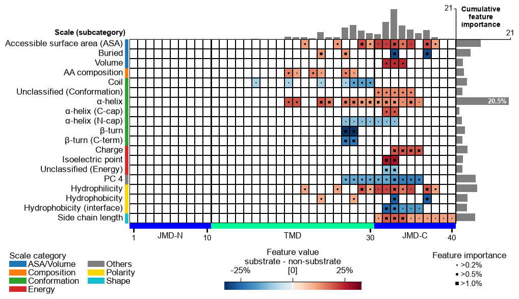
Visualise the whole signature as a feature map:
# MAP 2 -- the refined signature: the same run, after simplify. Fewer features and
# fewer subcategories than MAP 1, so the map speaks in coherent blocks. feature_map
# is an INSTANCE method and needs the feat_importance column added above.
aa.plot_settings(font_scale=0.65, weight_bold=False)
cpp_plot = aa.CPPPlot()
cpp_plot.feature_map(df_feat=df_feat, name_test="substrate", name_ref="non-substrate")
plt.tight_layout()
plt.show()
The two concepts the map makes visible
Where the signal sits: compositional vs positional. A feature’s
locality is not a strategy switch, it emerges from split_kws. Two
extremes answer different biological questions, and the map shows the
difference at a glance.
Compositional averages a whole part in one go,
Segment(1,1). The feature is amino-acid-composition-like and position-agnostic: it asks is this property higher in the TMD of substrates, anywhere in the TMD?Positional cuts a part into sub-segments (
n_split_max > 1), so a feature resolves to a sub-region: it asks where in the TMD?
Build each with get_split_kws() and hand it to
CPP(split_kws=...).
# Each variant below is the same three steps with a different split_kws:
# run CPP -> rank with a tree -> draw the map. Only split_kws changes.
def ranked(df_feat):
"""Add the feat_importance column that the feature map's bars need."""
X = sf.feature_matrix(features=df_feat["feature"], df_parts=df_parts)
tm = aa.TreeModel()
tm = tm.fit(X, labels=labels)
return tm.add_feat_importance(df_feat=df_feat)
def draw(df_feat):
"""Draw the canonical feature map for a signature."""
aa.plot_settings(font_scale=0.6, weight_bold=False)
aa.CPPPlot().feature_map(df_feat=df_feat, name_test="substrate",
name_ref="non-substrate")
plt.tight_layout()
plt.show()
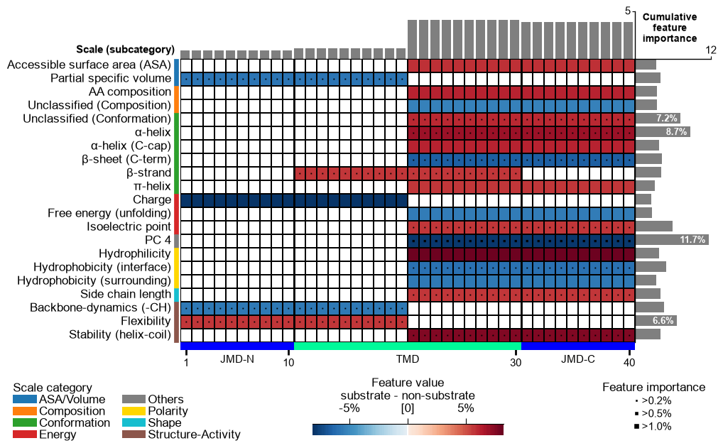
# MAP 3 -- COMPOSITIONAL: Segment(1,1) is one mean over the entire part.
split_kws_comp = sf.get_split_kws(split_types="Segment", n_split_min=1, n_split_max=1)
print("compositional split_kws:", split_kws_comp)
cpp = aa.CPP(df_parts=df_parts, split_kws=split_kws_comp)
df_feat_comp = ranked(cpp.run(labels=labels, n_filter=50, n_jobs=1))
draw(df_feat_comp)
compositional split_kws: {'Segment': {'n_split_min': 1, 'n_split_max': 1}}
# MAP 4 -- POSITIONAL: the same Segment split type, but cut into 2..6 sub-segments,
# so each feature covers a sub-region of a part instead of all of it.
split_kws_pos = sf.get_split_kws(split_types="Segment", n_split_min=2, n_split_max=6)
print("positional split_kws:", split_kws_pos)
cpp = aa.CPP(df_parts=df_parts, split_kws=split_kws_pos)
df_feat_pos = ranked(cpp.run(labels=labels, n_filter=50, n_jobs=1))
draw(df_feat_pos)
positional split_kws: {'Segment': {'n_split_min': 2, 'n_split_max': 6}}
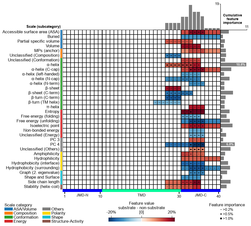
Compare the two maps above. The compositional map is built from
solid, part-wide bands: a cell spans all of jmd_n, tmd or
jmd_c, because that is exactly what one Segment(1,1) average
covers. The positional map breaks into narrow cells that concentrate
near the TMD/JMD-C boundary, saying not just which property separates
the groups but where it does. Same data, same scales: only the split
rule changed.
Split type: ``Segment`` vs ``Pattern``. Segment takes contiguous
chunks. Pattern instead takes fixed offsets counted from a terminus
(bounded by len_max), which catches an anchored or periodic
arrangement that a contiguous average washes out. PeriodicPattern is
the third type. The default split_kws uses all three, which is why
MAP 1 mixes them.
# MAP 5 -- PATTERN only: fixed offsets from a terminus rather than contiguous chunks.
split_kws_pat = sf.get_split_kws(split_types="Pattern")
print("pattern split_kws:", split_kws_pat)
cpp = aa.CPP(df_parts=df_parts, split_kws=split_kws_pat)
df_feat_pat = ranked(cpp.run(labels=labels, n_filter=50, n_jobs=1))
draw(df_feat_pat)
pattern split_kws: {'Pattern': {'steps': [3, 4], 'n_min': 2, 'n_max': 4, 'len_max': 15}}
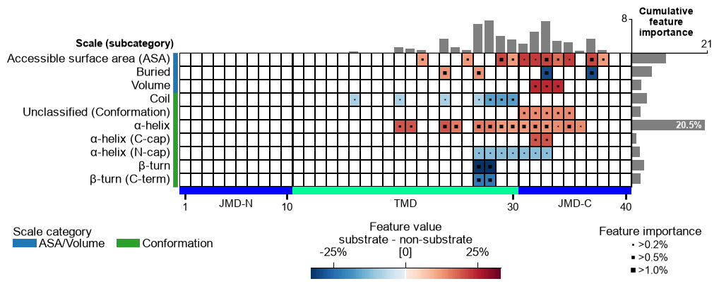
Reading one property family. Every scale carries an AAontology
category / subcategory, so the signature can be sliced to one
family of properties. The map is a lens on df_feat: filter the rows
and the same call shows that family alone, without the rest competing
for the eye. This is how you check whether a block you spotted in the
full map is really coherent.
# MAP 6 -- one property family: filter the refined signature to two AAontology
# categories. Swap the list to interrogate a different family.
categories = ["ASA/Volume", "Conformation"]
df_feat_cat = df_feat[df_feat["category"].isin(categories)]
print(f"{len(df_feat_cat)} of {len(df_feat)} features in {categories}")
aa.display_df(df=df_feat_cat, n_rows=8, show_shape=True)
draw(df_feat_cat)
18 of 35 features in ['ASA/Volume', 'Conformation']
DataFrame shape: (18, 15)
| feature | category | subcategory | scale_name | scale_description | abs_auc | abs_mean_dif | mean_dif | std_test | std_ref | p_val_mann_whitney | p_val_fdr_bh | positions | feat_importance | feat_importance_std | |
|---|---|---|---|---|---|---|---|---|---|---|---|---|---|---|---|
| 1 | TMD_C_JMD_C-Seg...2,3)-QIAN880106 | Conformation | α-helix | α-helix (middle) | Weights for alp...ejnowski, 1988) | 0.387000 | 0.121000 | 0.121000 | 0.069000 | 0.085000 | 0.000000 | 0.000000 | 27,28,29,30,31,32,33 | 7.927000 | 0.528000 |
| 7 | TMD_C_JMD_C-Pat...,15)-QIAN880107 | Conformation | α-helix | α-helix (middle) | Weights for alp...ejnowski, 1988) | 0.359000 | 0.158000 | 0.158000 | 0.081000 | 0.122000 | 0.000000 | 0.000001 | 25,28,32,35 | 5.273000 | 0.722000 |
| 8 | TMD_C_JMD_C-Seg...5,7)-LINS030101 | ASA/Volume | Volume | Accessible surface area (ASA) | Total accessibl...s et al., 2003) | 0.354000 | 0.237000 | 0.237000 | 0.146000 | 0.164000 | 0.000000 | 0.000001 | 32,33,34 | 2.712000 | 0.232000 |
| 9 | TMD_C_JMD_C-Pat...,12)-JANJ780101 | ASA/Volume | Accessible surface area (ASA) | ASA (folded protein) | Average accessi...n et al., 1978) | 0.348000 | 0.209000 | 0.209000 | 0.121000 | 0.164000 | 0.000000 | 0.000001 | 29,33,37 | 4.868000 | 0.529000 |
| 10 | TMD-Segment(11,12)-BEGF750103 | Conformation | β-turn | β-turn | Conformational ...in-Dirkx, 1975) | 0.343000 | 0.329000 | -0.329000 | 0.189000 | 0.247000 | 0.000000 | 0.000001 | 27,28 | 3.465000 | 0.508000 |
| 13 | TMD_C_JMD_C-Pat...4,8)-JANJ780102 | ASA/Volume | Buried | Buried | Percentage of b...n et al., 1978) | 0.340000 | 0.293000 | -0.293000 | 0.149000 | 0.246000 | 0.000000 | 0.000001 | 33,37 | 3.334000 | 0.685000 |
| 15 | TMD_C_JMD_C-Seg...4,5)-AURR980112 | Conformation | α-helix | α-helix | Normalized posi...ora-Rose, 1998) | 0.287000 | 0.137150 | 0.137150 | 0.099838 | 0.132861 | 0.000001 | 0.000001 | 33,34,35,36 | 1.617000 | 0.123000 |
| 16 | TMD_C_JMD_C-Per...4,2)-JANJ780101 | ASA/Volume | Accessible surface area (ASA) | ASA (folded protein) | Average accessi...n et al., 1978) | 0.336000 | 0.121000 | 0.121000 | 0.070000 | 0.107000 | 0.000000 | 0.000001 | 22,26,30,34,38 | 3.428000 | 0.674000 |
How to interpret. A few things to read off the feature map:
Output |
Non-expert reading |
|---|---|
high |
strong group-separating property |
positive |
property is higher in the test group in that region |
negative |
property is higher in the reference group |
a positional feature
(e.g. |
the signal depends on where in the part it occurs |
a whole-part |
a compositional (position-agnostic) difference |
a subcategory dominating the map |
that property family drives the separation |
Read the feature map as: rows = physicochemical properties (scale subcategories), columns = positions along the parts, colour = direction & strength of the difference, top bars = cumulative feature importance. A robust signature shows coherent blocks, not scattered single cells.
Because every scale belongs to an AAontology category/subcategory,
the signature reads as biology: a coherent block of high-abs_auc
features from one subcategory localised to a given part (e.g. the
tmd) says that property family, there, is what physicochemically
distinguishes the test group from the reference.
The six maps, and what each one isolates.
Map |
|
What it teaches |
|---|---|---|
|
default (all three split types) |
what |
|
same, after
|
the second CPP step: fewer, better-graded features saying the same thing |
|
|
part-wide bands: which property, position-agnostic |
|
|
narrow cells: where in the part the signal sits |
|
|
offsets from a terminus, not contiguous chunks |
|
filter |
whether a block is coherent within one AAontology family |
Maps 1 and 2 differ only by simplify; maps 3, 4 and 5 differ only by
split_kws; map 6 differs only by which rows of df_feat are
drawn. Everything else (data, labels, scales) is held fixed, so each map
isolates exactly one decision.
Key takeaways
The signature is the set of
Part-Split-Scalefeatures, not any single row: interpret coherent blocks (one subcategory, one region), and note whether they are compositional (whole-part) or positional (sub-region/pattern).mean_difcarries the direction (test minus reference) andabs_aucthe effect size;feat_importanceis an unsigned, group-level ranking signal: three complementary axes, not duplicates.A signature describes what separates the groups in this dataset; it is a hypothesis about determinants, so confirm stability before drawing biological conclusions.
Common mistakes.
Calling ``CPP(df_seq=…)`` or ``CPP().run(df_seq, labels)``:
CPPtakesdf_parts; build them withget_df_parts()first.Treating :meth:`~aaanalysis.CPPPlot.feature_map` as static: it is an instance method (
aa.CPPPlot().feature_map(...)), and it needs afeat_importancecolumn (add it withadd_feat_importance()).Over-reading a single feature: interpret the signature (blocks of related features), and check stability before drawing biological conclusions (see Protocol 9: Validate).
Using ``len(df_seq)`` for class sizes: use the
labelcolumn;load_dataset(..., n=N)returns2Nrows (N per class).
Next step. Continue with P2: Exploratory sequence analysis to explore one set of sequences without labels before contrasting groups.