ShapModel: Explaining with single-residue resolution

To enable explanations of sample-specific predictions at the single-residue level, we’ve developed a wrapper model around SHAP (SHapley Additive exPlanations). This explainable AI framework adopts a game-theoretic approach to elucidate the output of any machine learning model. Our ShapModel model, introduced in [Breimann25], fits multiple SHAP explainers and integrates their output to provide a robust estimate of feature impacts.

You will learn

• Tool: ShapModel

• Input: a feature matrix X, labels, and one or more model classes

• Output: per-sample SHAP feature impact (a df_feat impact column)

• Best used for: explaining individual predictions at single-residue resolution

• Related protocol: P9: Interpretability

• Related API: ShapModel

Obtaining Feature Impact

To illustrate, we’ll use an example dataset comprising γ-secretase substrates (n=63) and non-substrates (n=63) from [Breimann25]. We’ll explain the model’s prediction output for the Alzheimer’s disease-associated amyloid precursor protein (APP):

import aaanalysis as aa
aa.options["verbose"] = False
aa.options["random_state"] = 42

# Load dataset and respective features
df_seq = aa.load_dataset(name="DOM_GSEC")
labels = list(df_seq["label"])
df_feat = aa.load_features(name="DOM_GSEC")

# Show APP
aa.display_df(df=df_seq, n_rows=10, char_limit=25)

	entry	sequence	label	tmd_start	tmd_stop	jmd_n	tmd	jmd_c
1	P05067	MLPGLALLLLAA...NPTYKFFEQMQN	1	701	723	FAEDVGSNKG	AIIGLMVGGVVIATVIVITLVML	KKKQYTSIHH
2	P14925	MAGRARSGLLLL...YSAPLPKPAPSS	1	868	890	KLSTEPGSGV	SVVLITTLLVIPVLVLLAIVMFI	RWKKSRAFGD
3	P70180	MRSLLLFTFSAC...REDSIRSHFSVA	1	477	499	PCKSSGGLEE	SAVTGIVVGALLGAGLLMAFYFF	RKKYRITIER
4	Q03157	MGPTSPAARGQG...ENPTYRFLEERP	1	585	607	APSGTGVSRE	ALSGLLIMGAGGGSLIVLSLLLL	RKKKPYGTIS
5	Q06481	MAATGTAAAAAT...NPTYKYLEQMQI	1	694	716	LREDFSLSSS	ALIGLLVIAVAIATVIVISLVML	RKRQYGTISH
6	P35613	MAAALFVLLGFA...DKGKNVRQRNSS	1	323	345	IITLRVRSHL	AALWPFLGIVAEVLVLVTIIFIY	EKRRKPEDVL
7	P35070	MDRAARCSGASS...PINEDIEETNIA	1	119	141	LFYLRGDRGQ	ILVICLIAVMVVFIILVIGVCTC	CHPLRKRRKR
8	P09803	MGARCRSFSALL...KLADMYGGGEDD	1	711	733	GIVAAGLQVP	AILGILGGILALLILILLLLLFL	RRRTVVKEPL
9	P19022	MCRIAGALRTLL...KKLADMYGGGDD	1	724	746	RIVGAGLGTG	AIIAILLCIIILLILVLMFVVWM	KRRDKERQAK
10	P16070	MDKFWWHAAWGL...RNLQNVDMKIGV	1	650	672	GPIRTPQIPE	WLIILASLLALALILAVCIAVNS	RRRCGQKKKL

To fit the ShapModel, we fist need to create the feature matrix using the SequenceFeature.feat_matrix() method:

# Create feature matrix
sf = aa.SequenceFeature()
df_parts = sf.get_df_parts(df_seq=df_seq)
X = sf.feature_matrix(df_parts=df_parts, features=df_feat["feature"])

/Users/stephanbreimann/Programming/1Packages/aaanalysis/.claude/worktrees/pr222-fresh/aaanalysis/feature_engineering/_backend/cpp_run.py:143: UserWarning: CPP is using the Python kernel fallback — the compiled Cython extension is not available in this install. Output is bit-exact with the Cython path but ~2x slower. Reinstall via pip install --force-reinstall aaanalysis to fetch a prebuilt wheel.
  warnings.warn(

The difference of feature values between a selected protein (e.g., APP) and the reference dataset can be included into the feature DataFrame using the ShapModel.add_sample_mean_dif() method. This will create a new mean_dif_'name' column (e.g., ‘mean_dif_APP’):

sm = aa.ShapModel()
sm.fit(X, labels=labels)

# Add the feature value difference for the first protein (APP)
df_feat = sm.add_sample_mean_dif(X, labels=labels, df_feat=df_feat,
                                 sample_positions=0, names="APP")

/var/folders/sv/65tlch_10198qgmpwcp6408r0000gn/T/ipykernel_36922/2632148243.py:5: DeprecationWarning: 'sample_positions' is deprecated and will be removed in 1.2.0; use 'samples' instead.
  df_feat = sm.add_sample_mean_dif(X, labels=labels, df_feat=df_feat,

To add the sample-specific feature impact, use the ShapModel.add_feat_impact() method. This will create a new feat_impact_'name' column (e.g., ‘feat_impact_APP’):

# Add feature impacts for the first protein (APP)
df_feat = sm.add_feat_impact(df_feat=df_feat, sample_positions=0, names="APP")
aa.display_df(df=df_feat, n_rows=5)

/var/folders/sv/65tlch_10198qgmpwcp6408r0000gn/T/ipykernel_36922/41707308.py:2: DeprecationWarning: 'sample_positions' is deprecated and will be removed in 1.2.0; use 'samples' instead.
  df_feat = sm.add_feat_impact(df_feat=df_feat, sample_positions=0, names="APP")

	feature	category	subcategory	scale_name	scale_description	abs_auc	abs_mean_dif	mean_dif	std_test	std_ref	p_val_mann_whitney	p_val_fdr_bh	positions	feat_importance	feat_importance_std	mean_dif_APP	feat_impact_APP
1	TMD_C_JMD_C-Seg...3,4)-KLEP840101	Energy	Charge	Charge	Net charge (Kle...n et al., 1984)	0.244000	0.103666	0.103666	0.106692	0.110506	0.000000	0.000000	31,32,33,34,35	0.970400	1.438918	0.220635	0.980000
2	TMD_C_JMD_C-Seg...3,4)-FINA910104	Conformation	α-helix (C-cap)	α-helix termination	Helix terminati...n et al., 1991)	0.243000	0.085064	0.085064	0.098774	0.096946	0.000000	0.000000	31,32,33,34,35	0.000000	0.000000	0.193990	1.320000
3	TMD_C_JMD_C-Seg...6,9)-LEVM760105	Shape	Side chain length	Side chain length	Radius of gyrat... (Levitt, 1976)	0.233000	0.137044	0.137044	0.161683	0.176964	0.000000	0.000001	32,33	1.554800	2.109848	0.283275	1.710000
4	TMD_C_JMD_C-Seg...3,4)-HUTJ700102	Energy	Entropy	Entropy	Absolute entrop...Hutchens, 1970)	0.229000	0.098224	0.098224	0.106865	0.124608	0.000000	0.000001	31,32,33,34,35	3.111200	3.109955	0.162838	2.870000
5	TMD_C_JMD_C-Seg...6,9)-RADA880106	ASA/Volume	Volume	Accessible surface area (ASA)	Accessible surf...olfenden, 1988)	0.223000	0.095071	0.095071	0.114758	0.132829	0.000000	0.000002	32,33	0.000000	0.000000	0.189680	1.140000

Visualizing Feature Impact

Features can have either a positive (red) or negative (blue) impact, indicating whether they increase or decrease the model’s prediction output, respectively. Before visualizing impact of features, we need to obtain its sequence parts:

import matplotlib.pyplot as plt

# Get sequences parts for APP
seq_kws = sf.get_seq_kws(df_seq=df_seq, df_parts=df_parts, sample="P05067")   # Accession number of APP

To explain the feature impact with single-residue resolution, AAanalysis offers the following four types of visualizations: CPP-SHAP ranking plot, CPP-SHAP profile, CPP heatmap, CPP-SHAP heatmap. An overview is provided under Explainable AI Usage Principles

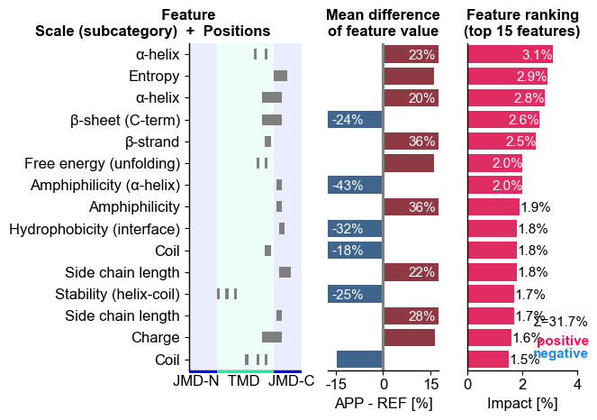
We can first show the feature ranking for a selected protein (‘Protein0’) using the CPPPlot.ranking() method, plotting SHAP analysis results by setting shap_plot=True:

# CPP-SHAP ranking plot
cpp_plot = aa.CPPPlot()
aa.plot_settings(short_ticks=True, weight_bold=False)
cpp_plot.ranking(df_feat=df_feat, shap_plot=True,
                 col_dif="mean_dif_APP", col_imp="feat_impact_APP",
                 name_test="APP")
plt.tight_layout()
plt.show()

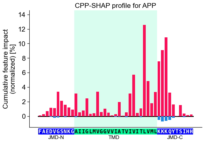
Show the specific CPP-SHAP Profile for the first Protein using the CPPPlot.profile() method with setting shap_plot=True:

# CPP-SHAP profile
aa.plot_settings(font_scale=0.9)
cpp_plot.profile(df_feat=df_feat, shap_plot=True,
                 col_imp="feat_impact_APP", **seq_kws)
plt.title("CPP-SHAP profile for APP")
plt.tight_layout()
plt.show()

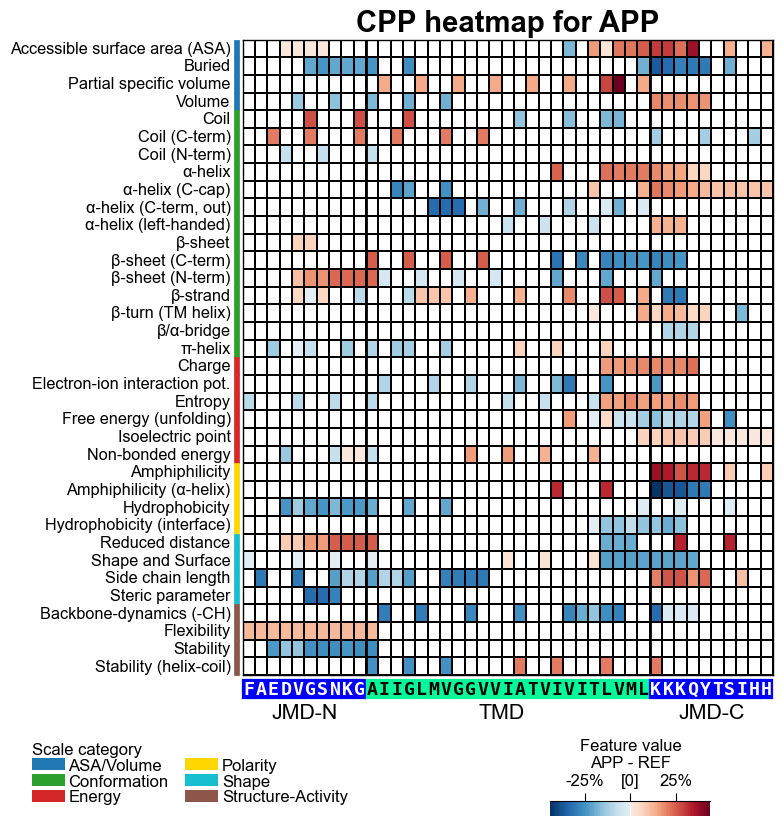
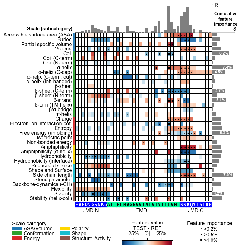
With the CPPPlot.heatmap() method we can visualize the sample-specific feature value difference and the feature impact per scale subcategory and residue position. Set shap_plot=True and provide the respective column with the mean difference and the feature impact:

# CPP heatmap (sample level)
fs = aa.plot_gcfs()
aa.plot_settings(font_scale=0.65, weight_bold=False)
cpp_plot.heatmap(df_feat=df_feat, shap_plot=True,
                 col_val="mean_dif_APP", **seq_kws, name_test="APP")
plt.title("CPP heatmap for APP", fontsize=fs+5, weight="bold")
plt.show()

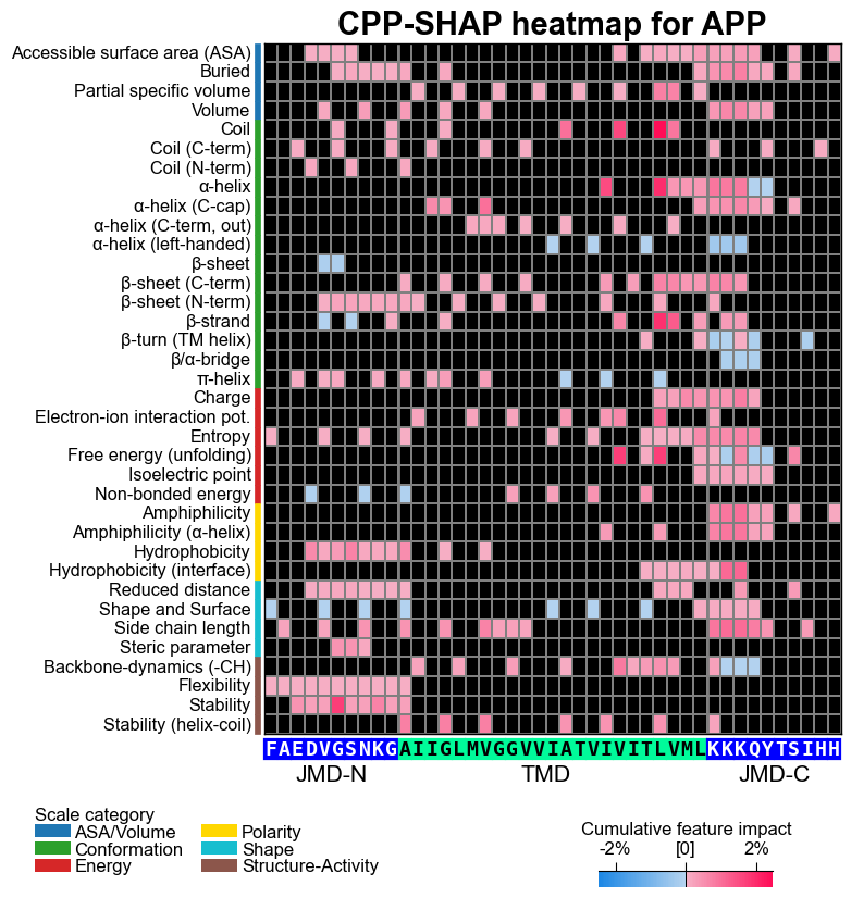
# CPP-SHAP heatmap (sample level)
cpp_plot.heatmap(df_feat=df_feat, shap_plot=True,
                 col_val="feat_impact_APP", **seq_kws)
plt.title("CPP-SHAP heatmap for APP", fontsize=fs+5, weight="bold")
plt.show()

To compare a specific sample, such as APP, with the positive test class, re-compute the feature value differences between the sample and the test set and visualize them as a CPP heatmap. We do not recommend using the feature map here, as feature impact or importance would not properly reflect the machine learning training context. Therefore, another colormap (‘PiYG_r’) is used to indicate the feature value differences.

# Add the feature value difference for the first protein (APP) against the test group
df_feat_app = sm.add_sample_mean_dif(X, labels=labels, df_feat=df_feat,
                                     sample_positions=0, names="APP", label_ref=1, drop=True)
# CPP-SHAP heatmap (sample level vs Test)
cpp_plot.heatmap(df_feat=df_feat_app, shap_plot=True,
                 col_val="mean_dif_APP", **seq_kws, name_test="APP", name_ref="Test set",
                 cmap="PiYG_r")
plt.title("CPP heatmap for APP vs Test set", fontsize=fs+5, weight="bold")
plt.show()

/var/folders/sv/65tlch_10198qgmpwcp6408r0000gn/T/ipykernel_36922/3186443046.py:2: DeprecationWarning: 'sample_positions' is deprecated and will be removed in 1.2.0; use 'samples' instead.
  df_feat_app = sm.add_sample_mean_dif(X, labels=labels, df_feat=df_feat,

You can create as well the feature map for individual samples. We first have the convert the feature impact into feature importance by simply taking their absolute values.

# Add feature importance
df_feat.insert(len(df_feat.T), "feat_importance_APP", [abs(x) for x in df_feat["feat_impact_APP"]])

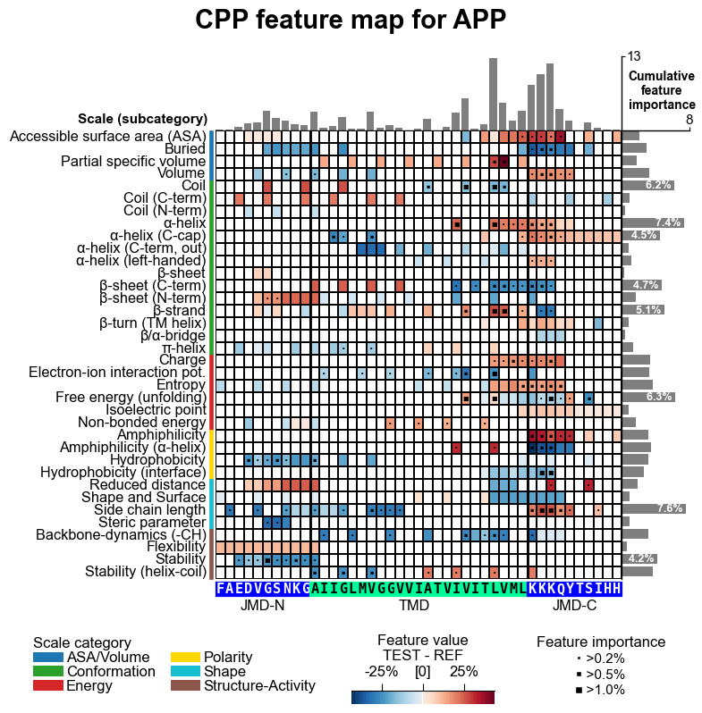
The feature map can be created using the CPPPlot.feature_map() method with providing the respective sequence parts and data columns. You can also set shap_plot=True and provide the respective column with the mean difference and the feature impact:

# CPP feature map (sample level with feature importance)
aa.plot_settings(font_scale=0.65, weight_bold=False)
cpp_plot.feature_map(df_feat=df_feat, col_val="mean_dif_APP", col_imp="feat_importance_APP", **seq_kws)
plt.suptitle("CPP feature map for APP", fontsize=fs+5, weight="bold")
plt.tight_layout()
plt.show()

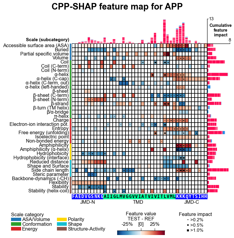
# CPP feature map (sample level with feature impact)
aa.plot_settings(font_scale=0.65, weight_bold=False)
cpp_plot.feature_map(df_feat=df_feat, col_val="mean_dif_APP", col_imp="feat_impact_APP", shap_plot=True, **seq_kws)
plt.suptitle("CPP-SHAP feature map for APP", fontsize=fs+5, weight="bold")
plt.tight_layout()
plt.show()

Details on the ShapModel class can be found in the ShapModel API. More information on explainable AI and how CPP and SHAP were combined are provided in the Explainable AI Usage Principles section.