P9: Interpretability

Turn a group-level CPP signature into a per-sample, single-residue explanation: SHAP and the CPP-SHAP heatmap. A CPP signature (P1) tells you which position-resolved physicochemical features separate a test group (label=1) from a reference group (label=0) on average. This protocol goes one level deeper: given that signature and a fitted tree model, ShapModel computes SHapley Additive exPlanations (SHAP) values, the signed contribution of each feature to one protein’s prediction score. The sample-level CPPPlot.heatmap (with shap_plot=True) then anchors those signed attributions onto the real residue positions of a single protein, so the explanation reads like “this protein’s TMD hydrophobicity at this position raised its substrate score” rather than an abstract feature index.

The signature is the group story; SHAP is the per-protein story. Feature importance is unsigned and group-level (how much does this feature matter overall?); feature impact is signed and sample-level (how much, and in which direction, did this feature push the score for this one protein?): red pushes toward the test class, blue toward the reference class. Read one sample’s impact as a local explanation, not as a new group claim.

We stay at the domain level (dataset prefix DOM_): the unit of comparison is the transmembrane-domain (TMD) part set of the gamma-secretase substrate task (DOM_GSEC), and we explain a single protein, APP, within it.

When to use it. Use this protocol when you already have a CPP signature (df_feat) plus a labelled feature matrix, and you want to explain a single protein’s prediction rather than the group as a whole. The biological question shifts from “what distinguishes substrates from non-substrates?” (determinant discovery, P1) to:

“Why does the model classify **this* protein (e.g. APP) as a gamma-secretase substrate, and where in its sequence do the decisive physicochemical differences act?”*

This is the protein-prediction analogue of a feature-attribution map (LIME / SHAP) in deep learning, but every attribution is anchored to an interpretable physicochemical scale and to a concrete residue position, not a black-box embedding dimension.

When not to use it. SHAP explains; it does not establish trust. Don’t use a single sample’s feature impact to make a group claim (“this scale defines substrates”): that is the signature’s job (P1). Don’t read it as proof the model generalizes: attributions are sample- and model-specific, and a model fit on a tiny set can attribute confidently to noise, so stability and controls come next (P10). And skip it entirely if you only need a ranked group signature: TreeModel.add_feat_importance already gives the unsigned, group-level ranking without fitting SHAP.

Input. This protocol receives its signature from P1: CPP signature and a fitted tree model from P7: Build an interpretable classifier. Concretely it needs:

• ``df_seq`` with a binary label column (test group = 1, reference group = 0). Here: the bundled DOM_GSEC set (gamma-secretase substrates vs. non-substrates), a domain-level task over the TMD and its flanking juxtamembrane (JMD) parts.

• ``df_feat``, the CPP signature from P1 (aa.load_features(name="DOM_GSEC") provides a precomputed signature here so this protocol stays self-contained).

• ``X``, the (n_samples, n_features) feature matrix built from df_feat["feature"] via SequenceFeature.feature_matrix.

• ``labels``, the class vector aligned to the rows of X.

We pick one protein to explain: APP (UniProt P05067), the Alzheimer’s-disease amyloid precursor protein and a canonical gamma-secretase substrate.

import aaanalysis as aa
import matplotlib.pyplot as plt

aa.options["verbose"] = False
aa.options["random_state"] = 42

# Small fixture: 50 per class (100 proteins total) keeps SHAP fitting fast
df_seq = aa.load_dataset(name="DOM_GSEC", n=50)
labels = df_seq["label"].to_list()

# CPP signature (from Protocol 1) and the feature matrix it indexes
df_feat = aa.load_features(name="DOM_GSEC")
sf = aa.SequenceFeature()
df_parts = sf.get_df_parts(df_seq=df_seq)
X = sf.feature_matrix(df_parts=df_parts, features=df_feat["feature"])

# Locate APP's row in X (non-substrates come first, so APP is NOT index 0; it sits at 50)
pos_app = list(df_seq["entry"]).index("P05067")

/Users/stephanbreimann/Programming/1Packages/aaanalysis/.claude/worktrees/pr222-fresh/aaanalysis/feature_engineering/_backend/cpp_run.py:143: UserWarning: CPP is using the Python kernel fallback — the compiled Cython extension is not available in this install. Output is bit-exact with the Cython path but ~2x slower. Reinstall via pip install --force-reinstall aaanalysis to fetch a prebuilt wheel.
  warnings.warn(

Run. Four steps, all on the real API (see the ShapModel tutorial for the function details):

1. Fit ``ShapModel``: trains the tree models and runs the SHAP explainer over several Monte-Carlo rounds, storing the per-sample attributions in shap_values.

2. Add the feature value difference for APP (add_sample_mean_dif): how APP’s feature values differ from the reference-group average.

3. Add the feature impact for APP (add_feat_impact): the signed, normalized SHAP attribution per feature.

4. Visualize with the sample-level CPPPlot methods (shap_plot=True).

# Fit ShapModel (pro feature; shap ships with the `pro` extra)
try:
    sm = aa.ShapModel(verbose=False, random_state=42)
    sm = sm.fit(X, labels=labels, n_rounds=3)  # 3 rounds is enough for a demo fixture
except ImportError as e:
    raise ImportError("ShapModel requires shap: pip install aaanalysis[pro]") from e

# Feature value difference: APP vs. the reference (non-substrate) group average
df_feat = sm.add_sample_mean_dif(X, labels=labels, df_feat=df_feat,
                                 sample_positions=pos_app, names="APP")

/var/folders/sv/65tlch_10198qgmpwcp6408r0000gn/T/ipykernel_36799/742728518.py:9: DeprecationWarning: 'sample_positions' is deprecated and will be removed in 1.2.0; use 'samples' instead.
  df_feat = sm.add_sample_mean_dif(X, labels=labels, df_feat=df_feat,

# Signed SHAP feature impact for APP (normalized to % of total absolute impact)
df_feat = sm.add_feat_impact(df_feat=df_feat, sample_positions=pos_app, names="APP")

aa.display_df(df=df_feat[["feature", "category", "mean_dif_APP", "feat_impact_APP"]], n_rows=8)

/var/folders/sv/65tlch_10198qgmpwcp6408r0000gn/T/ipykernel_36799/3501631186.py:2: DeprecationWarning: 'sample_positions' is deprecated and will be removed in 1.2.0; use 'samples' instead.
  df_feat = sm.add_feat_impact(df_feat=df_feat, sample_positions=pos_app, names="APP")

	feature	category	mean_dif_APP	feat_impact_APP
1	TMD_C_JMD_C-Seg...3,4)-KLEP840101	Energy	0.224000	0.660000
2	TMD_C_JMD_C-Seg...3,4)-FINA910104	Conformation	0.194644	1.280000
3	TMD_C_JMD_C-Seg...6,9)-LEVM760105	Shape	0.300050	1.570000
4	TMD_C_JMD_C-Seg...3,4)-HUTJ700102	Energy	0.177140	3.050000
5	TMD_C_JMD_C-Seg...6,9)-RADA880106	ASA/Volume	0.201494	1.300000
6	TMD_C_JMD_C-Seg...2,3)-KLEP840101	Energy	0.167146	1.250000
7	TMD_C_JMD_C-Seg...4,5)-FAUJ880109	Energy	0.146250	0.210000
8	TMD_C_JMD_C-Seg...3,4)-JANJ780101	ASA/Volume	0.373808	0.540000

# APP's sequence parts, used to anchor the plots to real residues
seq_kws = sf.get_seq_kws(df_seq=df_seq, df_parts=df_parts, sample="P05067")

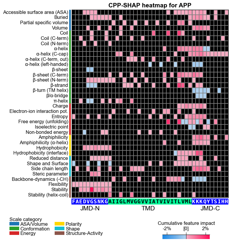
# CPP-SHAP heatmap (sample level): the headline figure.
# Each cell is the SIGNED SHAP impact of one feature on APP's substrate score,
# anchored to its real residue position and scale subcategory
# (red = pushes APP toward "substrate", blue = pushes toward "non-substrate").
fs = aa.plot_gcfs()
aa.plot_settings(font_scale=0.65, weight_bold=False)
cpp_plot = aa.CPPPlot()
fig, ax = cpp_plot.heatmap(df_feat=df_feat, shap_plot=True,
                           col_val="feat_impact_APP", name_test="APP", **seq_kws)
plt.title("CPP-SHAP heatmap for APP", fontsize=fs + 5, weight="bold")
plt.show()

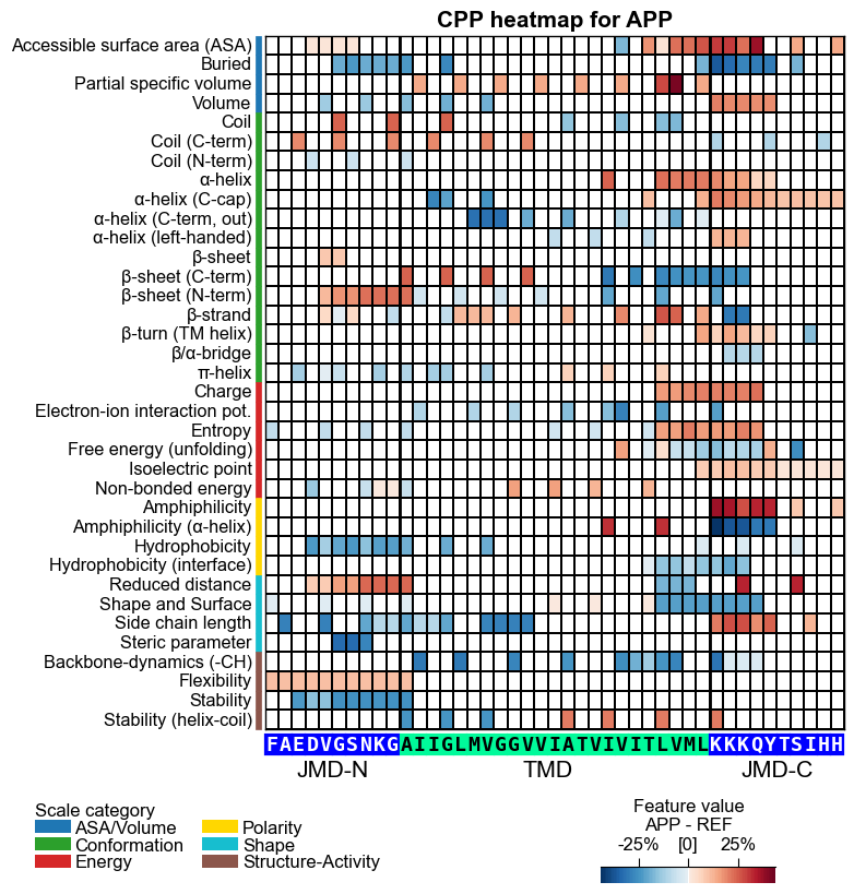
# CPP heatmap (sample level, mean-difference mode):
# each cell is APP's feature VALUE difference vs. the reference-group average,
# per scale subcategory and residue position (the complement to the impact heatmap above).
aa.plot_settings(font_scale=0.65, weight_bold=False)
fig, ax = cpp_plot.heatmap(df_feat=df_feat, shap_plot=True,
                           col_val="mean_dif_APP", name_test="APP", **seq_kws)
plt.title("CPP heatmap for APP", fontsize=fs + 5, weight="bold")
plt.show()

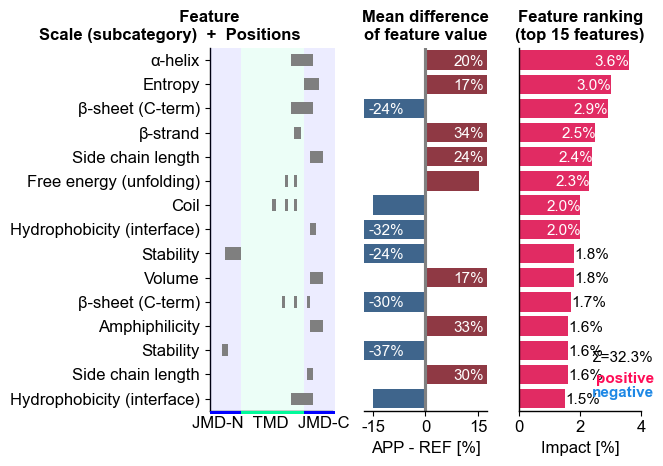
# CPP-SHAP ranking: top features for APP ordered by impact magnitude
aa.plot_settings(short_ticks=True, weight_bold=False)
fig, ax = cpp_plot.ranking(df_feat=df_feat, shap_plot=True,
                           col_dif="mean_dif_APP", col_imp="feat_impact_APP",
                           name_test="APP")
plt.tight_layout()
plt.show()

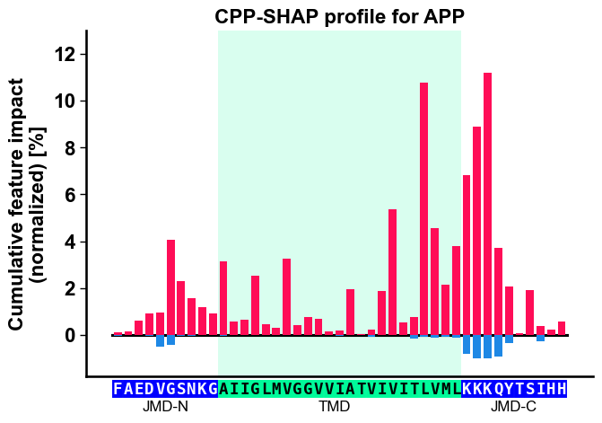
# CPP-SHAP profile: cumulative signed impact per residue position along APP
aa.plot_settings(font_scale=0.9)
fig, ax = cpp_plot.profile(df_feat=df_feat, shap_plot=True,
                           col_imp="feat_impact_APP", **seq_kws)
plt.title("CPP-SHAP profile for APP")
plt.tight_layout()
plt.show()

Output. df_feat gains two sample-level columns:

• mean_dif_APP: APP’s feature value difference vs. the reference-group average (sign = direction).

• feat_impact_APP: the signed SHAP attribution per feature, normalized so the absolute values sum to 100%.

Sample-level CPP-SHAP figures:

1. CPP-SHAP heatmap (impact mode): the headline figure; each cell is the signed SHAP impact of one feature on APP’s score (diverging colormap, red positive / blue negative), per scale subcategory and residue position.

2. CPP heatmap (mean-difference mode): each cell is APP’s feature value difference vs. the reference-group average, the complement that shows where APP physically differs.

3. Ranking: APP’s top features ordered by impact magnitude.

4. Profile: cumulative signed impact along the residue positions of APP’s JMD-N / TMD / JMD-C.

Every figure is anchored to APP’s actual sequence (jmd_n, tmd, jmd_c), so an attribution can be read off a specific residue.

How to interpret. A few things are happening in these figures. The heatmap row tells you which physicochemical subcategory and where along APP’s parts; the color tells you direction; the cumulative bars sum the signed impact per residue position. Read them like this:

Element	Reading
red bar / cell	feature’s SHAP impact is positive, pushing APP toward the test group (substrate)
blue bar / cell	feature’s SHAP impact is negative, pushing APP toward the reference group (non-substrate)
tall / saturated segment	feature contributes strongly in that direction
bar width at position x	cumulative impact from all features acting at residue position x
heatmap cell, mean-diff mode	APP’s feature value difference (test minus reference) at one position/scale
heatmap cell, impact mode	the signed contribution of that one feature to APP’s score

Worked reading (a recipe, not a claim about APP). This is the template you apply to whatever your own figure shows. For example, if you see a tall red bar over a TMD position whose row is a hydrophobicity subcategory, read it as: APP’s hydrophobicity is higher than the reference-group average there, and that excess hydrophobicity raised the classifier’s substrate score for APP. Swap in the actual subcategory, position, and color you observe: the figure, not this sentence, is the source of truth.

Key takeaways

• Coherent same-color blocks (e.g. red hydrophobicity across the TMD core) are a consistent, reliable local signal; isolated single cells are weak or conflicting evidence, so don’t over-read them.

• Sign agreement between mean_dif_APP and feat_impact_APP means APP follows the group trend the model learned (a confidence boost); a sign mismatch flags a possible outlier or a non-linear effect, so interpret with care.

• This is one protein’s local explanation. A high-impact feature for APP is not automatically a group determinant, so cross-check against the signature (P1) before generalizing.

Common mistakes.

• Calling ``add_feat_impact`` before ``fit``: shap_values is unset until ShapModel.fit runs, so impact cannot be computed.

• Assuming the sample is at index 0: with load_dataset(name="DOM_GSEC", n=50) the reference class (label 0) comes first, so APP sits at position 50, not 0. Always resolve the position from the entry (here list(df_seq["entry"]).index("P05067")).

• Mismatching ``shap_plot`` and the column: when shap_plot=True, col_val must be a per-sample column. Use feat_impact_'name' (signed) for the CPP-SHAP impact heatmap and mean_dif_'name' for the feature-value heatmap, not the group-level feat_importance (unsigned). The two are semantically opposite.

• Treating ``CPPPlot.heatmap`` as static: it is an instance method (aa.CPPPlot().heatmap(...)).

• Over-generalizing one sample: SHAP values are sample- and model-specific. A high-impact feature for APP does not mean it generalizes to all substrates; cross-check against the group signature (P1).

• Forgetting the ``pro`` extra: ShapModel needs shap (pip install aaanalysis[pro]).

Next step. P10: Validation (can I trust this?). Before reading a single sample’s explanation as biology, test the signature’s stability:

• Repeated cross-validation: refit CPP + ShapModel over random splits; do the SHAP rankings converge?

• Feature-drop tests: remove top-impact features one at a time; does performance degrade as expected?

• Shuffled-label controls: refit on permuted labels; genuine impacts should collapse to noise.

• Bootstrap confidence intervals: resample proteins within each class; do the attributions stay consistent?

See P10: Validation.