explain_features
- explain_features(df_feat, df_seq, labels, list_model_classes=None, label_target_class=1, samples=None, add_sample_mean_dif=False, label_ref=0, name_test='TEST', name_ref='REF', plot=True, random_state=None, n_jobs=None, verbose=False)[source]
Explain a feature set in one call: compute per-sample SHAP impact and draw the SHAP feature map.
A thin, stateless pro facade over the explicit primitive path. It rebuilds the feature matrix
Xfrom the feature identifiers indf_feat(viaSequenceFeature.get_df_parts()+SequenceFeature.feature_matrix()), fits aShapModel, attaches the per-sample SHAP feature impact todf_feat(viaShapModel.add_feat_impact()), and draws the SHAP-coloured feature map (CPPPlot.feature_map()withshap_plot=True). The defaults are byte-identical to writing those calls by hand.By default a single sample is explained: the
label_target_classsample the models predict most confidently — the most representative correct prediction. Passsamples(anentryname, a row position, or a list) to explain chosen sample(s) instead; the feature map then colours by the first requested sample’s impact and the impacts of all of them are added todf_feat.Warning
Experimental. This
aaanalysis.pipe(ap) golden pipeline is under active development; its API (signatures, defaults, return objects) may change between minor releases without the usual deprecation cycle. Pin a version if you depend on the current behaviour.- Parameters:
df_feat (pd.DataFrame, shape (n_features, n_feature_info)) – Feature DataFrame with a
featurecolumn of feature identifiers (e.g. fromCPP.run(),aaanalysis.pipe.find_features(), orload_features()).df_seq (pd.DataFrame, shape (n_samples, n_seq_info)) – Sequence DataFrame with the sequence/parts information, row-aligned to
labels. The feature matrix is rebuilt from it viaSequenceFeature.get_df_parts().labels (array-like, shape (n_samples,)) – Class labels for the samples (typically, 1=positive, 0=negative).
list_model_classes (list of Type[BaseEstimator], optional) – Prediction model classes passed to
ShapModel. IfNone, theShapModeldefault ([RandomForestClassifier, ExtraTreesClassifier]) is used.label_target_class (int, default=1) – The class label for which SHAP values are computed and the sample is auto-selected.
samples (int, str, list of int, list of str, or None) – Sample(s) to explain, given as row position(s) in the feature matrix or
entryname(s) fromdf_seq. IfNone, the most confidently predictedlabel_target_classsample is selected automatically.add_sample_mean_dif (bool, default=False) – If
True, also enrich the returneddf_featwith per-sample mean-difference columnsmean_dif_'name'(each explained sample’s feature value minus thelabel_refgroup average) alongside the SHAPfeat_impact_'name'columns, for the same sample(s) and names. This is the per-sample contrast a sample-level CPP-SHAP map/ranking is coloured by (viaShapModel.add_sample_mean_dif()); compute stays separate from plotting. DefaultFalseleaves the returned columns unchanged.label_ref (int, default=0) – Reference-group label whose per-feature average each sample is contrasted against for the
mean_dif_'name'columns. Used only whenadd_sample_mean_dif=True.name_test (str, default="TEST") – Name of the test (positive) group, shown on the feature map.
name_ref (str, default="REF") – Name of the reference (negative) group, shown on the feature map.
plot (bool, default=True) – If
True, draw the SHAP-coloured feature map and return itsAxes; ifFalse, skip the plot and returnNonein the figure slot.random_state (int, optional) – The seed used by the random number generator. If a positive integer, results of stochastic processes (the SHAP estimation and sample selection) are reproducible.
n_jobs (int, optional) – Number of CPU cores (>=1) for building the feature matrix. If
None, the optimized number is used.verbose (bool, default=False) – If
True, verbose progress information is printed.
- Returns:
df_feat_shap (pd.DataFrame, shape (n_features, n_feature_info+n)) –
df_featwith the per-sample SHAP feature impact added asfeat_impact_'name'column(s), plus per-samplemean_dif_'name'column(s) whenadd_sample_mean_dif=True.ax (matplotlib.axes.Axes or None) – The Axes of the SHAP-coloured feature map, or
Noneifplot=False.evals (None) – Always
None— explanation does no evaluation (keeps the uniform(results, figs, evals)pipeline return shape).
See also
ShapModelfor the underlying Monte Carlo SHAP estimation and feature impact.CPPPlot.feature_map()for the SHAP-coloured feature map (shap_plot=True).aaanalysis.pipe.find_features()for obtainingdf_feat(the feature discovery step).
Warning
This pipeline requires SHAP, which is automatically installed via
pip install aaanalysis[pro].
Examples
The
aaanalysis.pipe(ap) module provides high-level golden pipelines — stateless, one-call wrappers over the AAanalysis primitives.ap.explain_featuresis the pro explanation pipeline: given an existingdf_featand the sequences, it rebuilds the feature matrix, fits a :class:ShapModel, attaches the per-sample SHAP feature impact todf_feat, and draws the SHAP-coloured feature map. It returns the triple(df_feat_shap, ax, None)(explanation does no evaluation). It requiresaaanalysis[pro](SHAP).import matplotlib.pyplot as plt import aaanalysis as aa import aaanalysis.pipe as ap aa.options["verbose"] = False aa.plot_settings() # Sequences (df_seq) + labels and a discovered feature set (df_feat, e.g. from ap.find_features) df_seq = aa.load_dataset(name="DOM_GSEC", n=20) labels = df_seq["label"].to_list() df_feat = aa.load_features().head(25) aa.display_df(df_feat, n_rows=10, show_shape=True)
DataFrame shape: (25, 15)
feature category subcategory scale_name scale_description abs_auc abs_mean_dif mean_dif std_test std_ref p_val_mann_whitney p_val_fdr_bh positions feat_importance feat_importance_std 1 TMD_C_JMD_C-Seg...3,4)-KLEP840101 Energy Charge Charge Net charge (Kle...n et al., 1984) 0.244000 0.103666 0.103666 0.106692 0.110506 0.000000 0.000000 31,32,33,34,35 0.970400 1.438918 2 TMD_C_JMD_C-Seg...3,4)-FINA910104 Conformation α-helix (C-cap) α-helix termination Helix terminati...n et al., 1991) 0.243000 0.085064 0.085064 0.098774 0.096946 0.000000 0.000000 31,32,33,34,35 0.000000 0.000000 3 TMD_C_JMD_C-Seg...6,9)-LEVM760105 Shape Side chain length Side chain length Radius of gyrat... (Levitt, 1976) 0.233000 0.137044 0.137044 0.161683 0.176964 0.000000 0.000001 32,33 1.554800 2.109848 4 TMD_C_JMD_C-Seg...3,4)-HUTJ700102 Energy Entropy Entropy Absolute entrop...Hutchens, 1970) 0.229000 0.098224 0.098224 0.106865 0.124608 0.000000 0.000001 31,32,33,34,35 3.111200 3.109955 5 TMD_C_JMD_C-Seg...6,9)-RADA880106 ASA/Volume Volume Accessible surface area (ASA) Accessible surf...olfenden, 1988) 0.223000 0.095071 0.095071 0.114758 0.132829 0.000000 0.000002 32,33 0.000000 0.000000 6 TMD_C_JMD_C-Seg...2,3)-KLEP840101 Energy Charge Charge Net charge (Kle...n et al., 1984) 0.222000 0.058671 0.058671 0.064895 0.069547 0.000000 0.000001 27,28,29,30,31,32,33 0.000000 0.000000 7 TMD_C_JMD_C-Seg...4,5)-FAUJ880109 Energy Isoelectric point Number hydrogen bond donors Number of hydro...e et al., 1988) 0.215000 0.146661 0.146661 0.174609 0.188034 0.000000 0.000004 33,34,35,36 1.032400 1.510722 8 TMD_C_JMD_C-Seg...3,4)-JANJ780101 ASA/Volume Accessible surface area (ASA) ASA (folded protein) Average accessi...n et al., 1978) 0.215000 0.124317 0.124317 0.166309 0.153364 0.000000 0.000004 31,32,33,34,35 1.080400 1.296094 9 TMD_C_JMD_C-Seg...,10)-WILM950103 Polarity Hydrophobicity (interface) Hydrophobicity (interface) Hydrophobicity ...e et al., 1995) 0.212000 0.141305 -0.141305 0.168603 0.217235 0.000000 0.000005 33,34 1.747200 2.150664 10 TMD_C_JMD_C-Seg...6,9)-AURR980110 Conformation α-helix α-helix (middle) Normalized posi...ora-Rose, 1998) 0.211000 0.125350 0.125350 0.160819 0.174121 0.000000 0.000005 32,33 1.788800 2.700803 By default a single sample is explained: the
label_target_classsample the models predict most confidently — the most representative correct prediction. The per-sample SHAP impact is added todf_featas afeat_impact_'entry'column, and the feature map colours each feature by that signed impact.random_statemakes the SHAP estimation and the sample selection reproducible;n_jobsparallelizes the feature-matrix build:df_shap, ax, evals = ap.explain_features(df_feat, df_seq, labels, random_state=42, n_jobs=1) impact_cols = [c for c in df_shap.columns if c.startswith("feat_impact_")] print("impact columns:", impact_cols, "| evals:", evals) plt.tight_layout() plt.show()
/Users/stephanbreimann/Programming/1Packages/wt-412-explain-meandif/aaanalysis/feature_engineering/_backend/cpp_run.py:164: UserWarning: CPP is using the Python kernel fallback — the compiled Cython extension is not available in this install. Output is bit-exact with the Cython path but ~2x slower. Reinstall via pip install --force-reinstall aaanalysis to fetch a prebuilt wheel.
  warnings.warn(
impact columns: ['feat_impact_Q06481'] | evals: None
Pass
samplesto explain chosen sample(s) instead of auto-selecting — anentryname, a row position, or a list of them.label_target_classsets the class SHAP targets,list_model_classesoverrides the prediction models, andplot=Falseskips the figure (axis thenNone). Here we explain two named proteins with an explicit model list:from sklearn.ensemble import RandomForestClassifier, ExtraTreesClassifier entries = df_seq["entry"].iloc[:2].to_list() df_shap, ax, _ = ap.explain_features(df_feat, df_seq, labels, samples=entries, label_target_class=1, list_model_classes=[RandomForestClassifier, ExtraTreesClassifier], plot=False, random_state=42, n_jobs=1, verbose=False) cols = ["feature"] + [c for c in df_shap.columns if c.startswith("feat_impact_")] aa.display_df(df_shap[cols], n_rows=10, show_shape=True)
DataFrame shape: (25, 3)
feature feat_impact_Q14802 feat_impact_Q86UE4 1 TMD_C_JMD_C-Seg...3,4)-KLEP840101 -0.110000 -2.300000 2 TMD_C_JMD_C-Seg...3,4)-FINA910104 -0.520000 -2.370000 3 TMD_C_JMD_C-Seg...6,9)-LEVM760105 -7.850000 -4.720000 4 TMD_C_JMD_C-Seg...3,4)-HUTJ700102 -5.370000 -4.380000 5 TMD_C_JMD_C-Seg...6,9)-RADA880106 -9.310000 -5.250000 6 TMD_C_JMD_C-Seg...2,3)-KLEP840101 0.090000 -2.490000 7 TMD_C_JMD_C-Seg...4,5)-FAUJ880109 -6.880000 -7.960000 8 TMD_C_JMD_C-Seg...3,4)-JANJ780101 -1.560000 -0.650000 9 TMD_C_JMD_C-Seg...,10)-WILM950103 -7.300000 -6.520000 10 TMD_C_JMD_C-Seg...6,9)-AURR980110 -11.270000 -0.040000 Set
add_sample_mean_dif=Trueto also enrichdf_featwith per-sample mean-difference columnsmean_dif_'name'(each sample’s feature value minus thelabel_refgroup average) alongside the SHAPfeat_impact_'name'columns. This is the per-sample contrast a sample-level CPP-SHAP map or ranking is coloured by, kept separate from plotting;label_refchooses the reference group:df_shap, ax, _ = ap.explain_features(df_feat, df_seq, labels, samples=df_seq["entry"].iloc[0], add_sample_mean_dif=True, label_ref=0, plot=False, random_state=42, n_jobs=1) name = df_seq["entry"].iloc[0] cols = ["feature", f"feat_impact_{name}", f"mean_dif_{name}"] aa.display_df(df_shap[cols], n_rows=10, show_shape=True)
DataFrame shape: (25, 3)
feature feat_impact_Q14802 mean_dif_Q14802 1 TMD_C_JMD_C-Seg...3,4)-KLEP840101 -0.110000 0.085000 2 TMD_C_JMD_C-Seg...3,4)-FINA910104 -0.520000 0.078780 3 TMD_C_JMD_C-Seg...6,9)-LEVM760105 -7.850000 0.092233 4 TMD_C_JMD_C-Seg...3,4)-HUTJ700102 -5.370000 0.045490 5 TMD_C_JMD_C-Seg...6,9)-RADA880106 -9.310000 0.073717 6 TMD_C_JMD_C-Seg...2,3)-KLEP840101 0.090000 0.060716 7 TMD_C_JMD_C-Seg...4,5)-FAUJ880109 -6.880000 -0.040625 8 TMD_C_JMD_C-Seg...3,4)-JANJ780101 -1.560000 0.023330 9 TMD_C_JMD_C-Seg...,10)-WILM950103 -7.300000 0.183475 10 TMD_C_JMD_C-Seg...6,9)-AURR980110 -11.270000 -0.005536 With
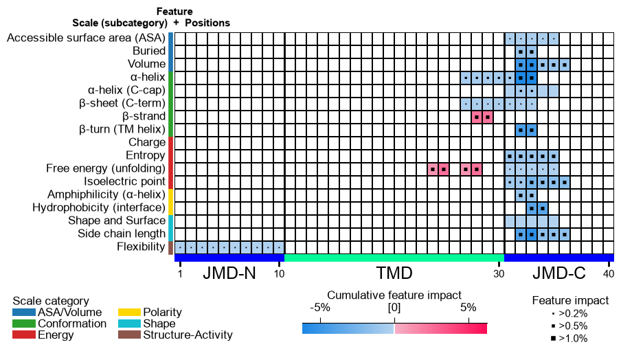
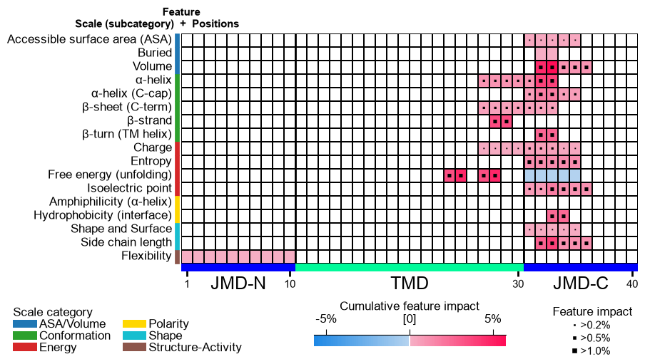
plot=Truethe SHAP-coloured feature map is drawn for the first requested sample;name_testandname_reflabel the two groups. The returnedaxis the feature-mapAxes:df_shap, ax, _ = ap.explain_features(df_feat, df_seq, labels, samples=df_seq["entry"].iloc[0], name_test="SUBSTRATE", name_ref="NON-SUB", plot=True, random_state=42, n_jobs=1) plt.tight_layout() plt.show()