CPPPlot.feature
- CPPPlot.feature(feature, feat_rank=1, *, df_seq, labels, label_test=1, label_ref=0, ax=None, figsize=(5.6, 4.8), names_to_show=None, name_test='TEST', name_ref='REF', color_test='tab:green', color_ref='tab:gray', show_seq=False, show_title=True, title_wrap_width=45, histplot=False, fontsize_mean_dif=15, fontsize_name_test=13, fontsize_name_ref=13, fontsize_names_to_show=11, alpha_hist=0.1, alpha_dif=0.2)[source]
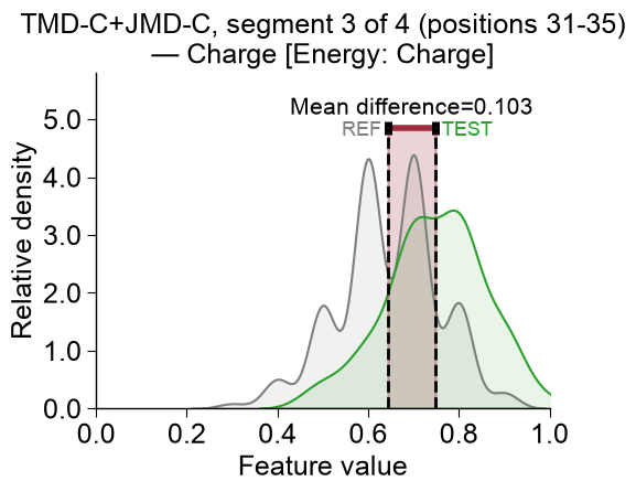
Plot distributions of Comparative Physicochemical Profiling (CPP) feature values for test and reference datasets highlighting their mean difference.
Introduced in [Breimann24a], a CPP feature is defined as a Part-Split-Scale combination. For a sample, a feature value is computed in three steps:
Part Selection: Identify a specific sequence part.
Part-Splitting: Divide the selected part into subsequences, creating a Part-Split combination.
Scale Value Assignment: For each amino acid in the Part-Split subsequence, assign its corresponding scale value and calculate the average, which is termed the feature value.
Added in version 0.1.0.
- Parameters:
feature (str, list of str, or pd.DataFrame) – The feature(s) to plot, given as a single
PART-SPLIT-SCALEfeature id, a list of such ids, or a feature DataFrame (df_feat) whosefeaturecolumn supplies the ids. When more than one feature is provided,feat_rankselects which one is plotted. The order is taken as given (pre-sort withTreeModel.add_feat_importance()usingsort=Trueto place the most important feature first).feat_rank (int, default=1) – 1-based rank selecting which feature to plot when
featureholds more than one (1= first/top,2= second, …). Must be between 1 and the number of provided features. For a single feature it must be1.df_seq (pd.DataFrame, shape (n_samples, n_seq_info)) – DataFrame containing an
entrycolumn with unique protein identifiers and sequence information in a distinct Position-based, Part-based, Sequence-based, or Sequence-TMD-based format.labels (array-like, shape (n_samples,)) – Class labels for samples in sequence DataFrame (typically, test=1, reference=0).
label_test (int, default=1,) – Class label of test group in
labels.label_ref (int, default=0,) – Class label of reference group in
labels.ax (Axes, optional) – Pre-defined Axes object to plot on. If
None, a new Axes object is created.figsize (tuple, default=(5.6, 4.8)) – Figure dimensions (width, height) in inches.
names_to_show (list of str, optional) – Names of specific samples from
df_seqto highlight on plot. ‘name’ column must be given indf_seqifnames_to_showis notNone.name_test (str, default="TEST") – Name for the test dataset.
name_ref (str, default="REF") – Name for the reference dataset.
color_test (str, default="tab:green") – Color for the test dataset.
color_ref (str, default="tab:gray") – Color for the reference dataset.
show_seq (bool, default=False) – If
True, show sequence of samples selected vianames_to_show.show_title (bool, default=True) – If
True, set the plot title to the feature’s human-readable description (seeSequenceFeature.get_feature_descriptions()), line-wrapped attitle_wrap_width. A subsequentplt.title(...)/ax.set_title(...)call still overrides it.title_wrap_width (int, default=45) – Maximum line width (in characters, >0) for wrapping the
show_titledescription.histplot (bool, default=False) – If
True, plot a histogram. IfFalse, plot a kernel density estimate (KDE) plot.fontsize_mean_dif (int or float, default=15) – Font size (>0) for displayed mean difference text.
fontsize_name_test (int or float, default=13) – Font size (>0) for the name of the test dataset.
fontsize_name_ref (int or float, default=13) – Font size (>0) for the name of the reference dataset.
fontsize_names_to_show (int or float, default=11) – Font size (>0) for the names selected via
names_to_show.alpha_hist (int or float, default=0.1) – The transparency alpha value [0-1] for the histogram distributions.
alpha_dif (int or float, default=0.2) – The transparency alpha value [0-1] for the mean difference area.
- Returns:
fig (Figure) – Figure object containing the plot.
ax (Axes) – CPP feature plot axes object.
Notes
Returned as a
(fig, ax)pair (seeCPPPlotfor the shared return contract).
See also
SequenceFeaturefor details on CPP feature concept.SequenceFeature.get_df_parts()for details on formats ofdf_seq.The internally used
seaborn.histplot()andseaborn.kdeplot()functions.
Examples
To demonstrate the
CCPPlot().feature()method, we load theDOM_GSECexample dataset (see [Breimann25]):import matplotlib.pyplot as plt import aaanalysis as aa aa.options["verbose"] = False df_seq = aa.load_dataset(name="DOM_GSEC_PU") labels = df_seq["label"].to_list() labels = [0 if x == 2 else x for x in labels] # Adjust labels
For any feature, we can display the distribution of feature values for a test and a reference dataset, provided by the
df_seqand the correspondinglabelsparameters. The feature has to be a validPart-Split-Scalecombination (scales are given by their AAindex id):# This feature creates the average volume over the entire TMD sequence feature = "TMD-Segment(1,1)-GRAR740103" cpp_plot = aa.CPPPlot() aa.plot_settings(font_scale=1) cpp_plot.feature(feature=feature, df_seq=df_seq, labels=labels) plt.title("Average TMD Volume (GRAR740103)") plt.tight_layout() plt.show()

We can now load the respective feature set for the
DOM_GSEC_PUdataset:sf = aa.SequenceFeature() df_parts = sf.get_df_parts(df_seq=df_seq) df_feat = aa.load_features(name="DOM_GSEC") aa.display_df(df_feat, n_rows=15)
feature category subcategory scale_name scale_description abs_auc abs_mean_dif mean_dif std_test std_ref p_val_mann_whitney p_val_fdr_bh positions feat_importance feat_importance_std 1 TMD_C_JMD_C-Seg...3,4)-KLEP840101 Energy Charge Charge Net charge (Kle...n et al., 1984) 0.244000 0.103666 0.103666 0.106692 0.110506 0.000000 0.000000 31,32,33,34,35 0.970400 1.438918 2 TMD_C_JMD_C-Seg...3,4)-FINA910104 Conformation α-helix (C-cap) α-helix termination Helix terminati...n et al., 1991) 0.243000 0.085064 0.085064 0.098774 0.096946 0.000000 0.000000 31,32,33,34,35 0.000000 0.000000 3 TMD_C_JMD_C-Seg...6,9)-LEVM760105 Shape Side chain length Side chain length Radius of gyrat... (Levitt, 1976) 0.233000 0.137044 0.137044 0.161683 0.176964 0.000000 0.000001 32,33 1.554800 2.109848 4 TMD_C_JMD_C-Seg...3,4)-HUTJ700102 Energy Entropy Entropy Absolute entrop...Hutchens, 1970) 0.229000 0.098224 0.098224 0.106865 0.124608 0.000000 0.000001 31,32,33,34,35 3.111200 3.109955 5 TMD_C_JMD_C-Seg...6,9)-RADA880106 ASA/Volume Volume Accessible surface area (ASA) Accessible surf...olfenden, 1988) 0.223000 0.095071 0.095071 0.114758 0.132829 0.000000 0.000002 32,33 0.000000 0.000000 6 TMD_C_JMD_C-Seg...2,3)-KLEP840101 Energy Charge Charge Net charge (Kle...n et al., 1984) 0.222000 0.058671 0.058671 0.064895 0.069547 0.000000 0.000001 27,28,29,30,31,32,33 0.000000 0.000000 7 TMD_C_JMD_C-Seg...4,5)-FAUJ880109 Energy Isoelectric point Number hydrogen bond donors Number of hydro...e et al., 1988) 0.215000 0.146661 0.146661 0.174609 0.188034 0.000000 0.000004 33,34,35,36 1.032400 1.510722 8 TMD_C_JMD_C-Seg...3,4)-JANJ780101 ASA/Volume Accessible surface area (ASA) ASA (folded protein) Average accessi...n et al., 1978) 0.215000 0.124317 0.124317 0.166309 0.153364 0.000000 0.000004 31,32,33,34,35 1.080400 1.296094 9 TMD_C_JMD_C-Seg...,10)-WILM950103 Polarity Hydrophobicity (interface) Hydrophobicity (interface) Hydrophobicity ...e et al., 1995) 0.212000 0.141305 -0.141305 0.168603 0.217235 0.000000 0.000005 33,34 1.747200 2.150664 10 TMD_C_JMD_C-Seg...6,9)-AURR980110 Conformation α-helix α-helix (middle) Normalized posi...ora-Rose, 1998) 0.211000 0.125350 0.125350 0.160819 0.174121 0.000000 0.000005 32,33 1.788800 2.700803 11 TMD_C_JMD_C-Seg...2,3)-AURR980110 Conformation α-helix α-helix (middle) Normalized posi...ora-Rose, 1998) 0.211000 0.077355 0.077355 0.102965 0.107453 0.000000 0.000005 27,28,29,30,31,32,33 3.048800 3.623912 12 TMD_C_JMD_C-Seg...3,4)-JANJ790102 Energy Free energy (unfolding) Transfer free e...(TFE) to inside Transfer free e...y (Janin, 1979) 0.206000 0.111462 -0.111462 0.159718 0.144989 0.000000 0.000009 31,32,33,34,35 0.000000 0.000000 13 TMD_C_JMD_C-Seg...6,9)-CHOC760103 ASA/Volume Buried Buried Proportion of r...(Chothia, 1976) 0.205000 0.125868 -0.125868 0.172165 0.188333 0.000000 0.000009 32,33 0.000000 0.000000 14 TMD_C_JMD_C-Seg...4,5)-LEVM760105 Shape Side chain length Side chain length Radius of gyrat... (Levitt, 1976) 0.204000 0.105513 0.105513 0.132849 0.145219 0.000000 0.000009 33,34,35,36 1.992000 2.929460 15 TMD_C_JMD_C-Seg...6,9)-DESM900102 Polarity Amphiphilicity (α-helix) Membrane preference Average membran...i et al., 1990) 0.200000 0.132693 -0.132693 0.184359 0.209008 0.000000 0.000015 32,33 0.000000 0.000000 We can plot the feature value distributions for the test and the reference datasets for the best feature using the
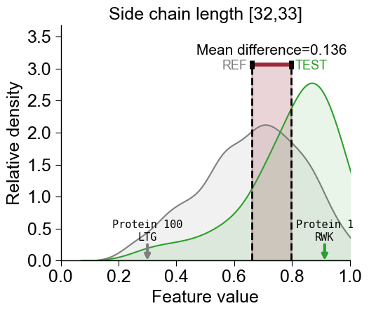
CCPPlot().feature()method. You need to provide the CPPfeatureid (Part-Split-Scalecombination), thedf_seqDataFrame, and its respectivelabels:list_features = df_feat["feature"].to_list() cpp_plot = aa.CPPPlot() aa.plot_settings(font_scale=1) cpp_plot.feature(feature=list_features[0], df_seq=df_seq, labels=labels) plt.tight_layout() plt.show()
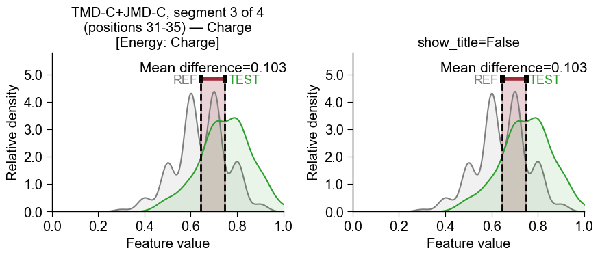
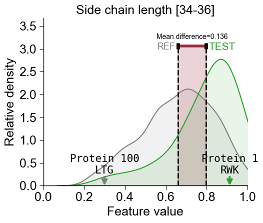
By default the plot title is the feature’s human-readable description (from
SequenceFeature().get_feature_descriptions()), line-wrapped attitle_wrap_width. Narrow or widen the wrap, or turn the title off withshow_title=False(then set your own withplt.title(...)):aa.plot_settings(font_scale=0.8) fig, axes = plt.subplots(1, 2, figsize=(9, 4)) cpp_plot.feature(feature=df_feat, df_seq=df_seq, labels=labels, feat_rank=1, ax=axes[0], title_wrap_width=30) cpp_plot.feature(feature=df_feat, df_seq=df_seq, labels=labels, feat_rank=1, ax=axes[1], show_title=False) axes[1].set_title("show_title=False") plt.tight_layout() plt.show()
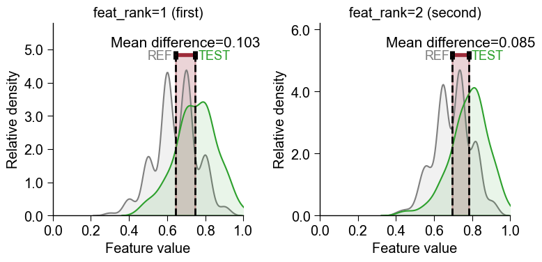
Instead of extracting a single feature id, you can pass a list of features or the whole feature DataFrame (
df_feat) directly tofeatureand choose which one to plot with the 1-basedfeat_rankparameter (feat_rank=1plots the first/top feature,feat_rank=2the second, …). The features are taken in the given order, so rankdf_featfirst withTreeModel.add_feat_importance(sort=True)to makefeat_rank=1the most important feature:# Pass df_feat directly and pick the feature by 1-based rank (no manual id extraction) aa.plot_settings(font_scale=0.8) fig, axes = plt.subplots(1, 2, figsize=(8, 4)) cpp_plot.feature(feature=df_feat, df_seq=df_seq, labels=labels, feat_rank=1, ax=axes[0]) cpp_plot.feature(feature=df_feat, df_seq=df_seq, labels=labels, feat_rank=2, ax=axes[1]) axes[0].set_title("feat_rank=1 (first)") axes[1].set_title("feat_rank=2 (second)") plt.tight_layout() plt.show()
Test vs Reference Dataset
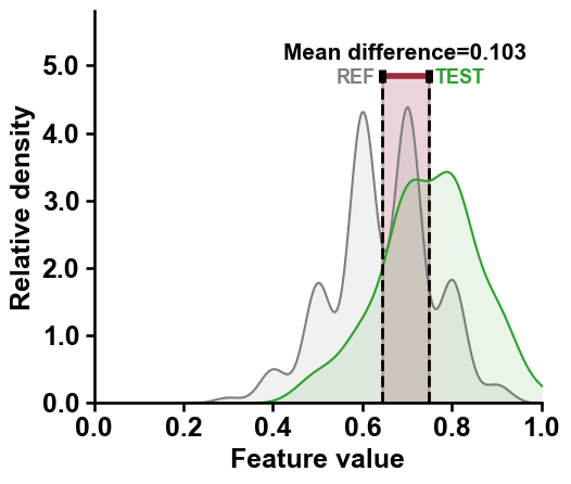
The distributions for the test dataset (
TEST, green) and the reference dataset (REF, gray) are compared by highlighted the difference of the mean values (calledMean difference).To use the shorter feature name as the title instead of the default description, override it with the
SequenceFeature().get_feature_names()method:sf = aa.SequenceFeature() feature_names = sf.get_feature_names(features=list_features) cpp_plot.feature(feature=list_features[0], df_seq=df_seq, labels=labels) plt.title(feature_names[0]) plt.tight_layout() plt.show()

You can use the
axparameter to create subplots for displaying multiple features:aa.plot_settings(font_scale=0.8) # Create subplots fig, axes = plt.subplots(1, 2, figsize=(8, 4)) cpp_plot.feature(ax=axes[0], feature=list_features[2], df_seq=df_seq, labels=labels) cpp_plot.feature(ax=axes[1], feature=list_features[12], df_seq=df_seq, labels=labels) axes[0].set_title(feature_names[2]) axes[1].set_title(feature_names[12]) plt.tight_layout() plt.show()

Positive vs Negative Mean Difference
The mean difference of feature values can be either positive or negative:
Positive (indicated in red) means that the feature values of the test class are higher in average (e.g., left plot).
Negative (indicated in blue) means that the feature values of the test class are lower in average (e.g., left plot).
You can customize the plot by changing the
figsize, dataset names (vianame_testandname_ref), or dataset colors (viacolor_testandcolor_ref):aa.plot_settings() cpp_plot.feature(feature=list_features[2], df_seq=df_seq, labels=labels, figsize=(5, 4), name_test="Test data", name_ref="Reference data", color_test="tab:orange", color_ref="tab:blue") plt.title(feature_names[2]) plt.tight_layout() plt.show()

You change the density plot to a histogram by setting
histplot=Truecpp_plot.feature(feature=list_features[2], df_seq=df_seq, labels=labels, histplot=True) plt.title(feature_names[2]) plt.tight_layout() plt.show()

Adjust the transparency (alpha value) of the histogram and the mean difference using the
alpha_hist(default=0.1) andalpha_dif(default=0.2) parameters:cpp_plot.feature(feature=list_features[2], df_seq=df_seq, labels=labels, alpha_dif=0.5, alpha_hist=0.7) plt.title(feature_names[2]) plt.tight_layout() plt.show()
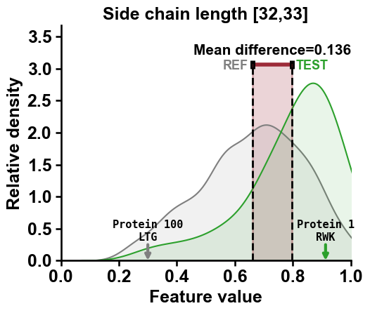
To highlight samples within the distributions, the
df_seqDataFrame needs to contain anamecolumn. Selected names from this column are displayed if provided via thenames_to_showparameter:df_seq["name"] = [f"Protein {i}" for i in range(len(df_seq))] cpp_plot.feature(feature=list_features[2], df_seq=df_seq, labels=labels, names_to_show=["Protein 1", "Protein 100"]) plt.title(feature_names[2]) plt.tight_layout() plt.show()
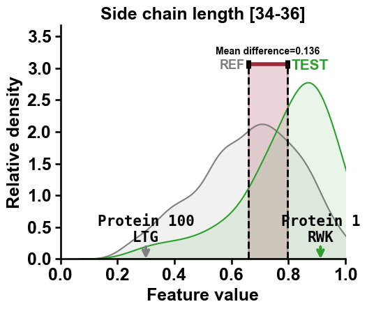
You can show the sub-sequence for the
Part-Splitcombination of the selected proteins by settingshow_seq=True:df_seq["name"] = [f"Protein {i}" for i in range(len(df_seq))] cpp_plot.feature(feature=list_features[2], df_seq=df_seq, labels=labels, names_to_show=["Protein 1", "Protein 100"], show_seq=True) plt.title(feature_names[2]) plt.tight_layout() plt.show()
Following parameters are provided to adjust the font size:
fontsize_mean_dif(default=15),fontsize_name_test(default=13),fontsize_name_ref(default=13), andfontsie_names_to_show(default=11):cpp_plot.feature(feature=list_features[2], df_seq=df_seq, labels=labels, names_to_show=["Protein 1", "Protein 100"], show_seq=True, fontsize_mean_dif=10, fontsize_name_test=15, fontsize_name_ref=13, fontsize_names_to_show=15) # Adjust the feature name for the TMD length feature_names = sf.get_feature_names(list_features[2], tmd_len=23) plt.title(feature_names[0]) plt.tight_layout() plt.show()
Further parameters.
CPPPlot.featurealso accepts:label_test— Class label of test group inlabels;label_ref— Class label of reference group inlabels.# Further parameters: label_test / label_ref name the two groups in labels (default 1 / 0) import matplotlib.pyplot as plt cpp_plot.feature(feature=list_features[0], df_seq=df_seq, labels=labels, label_test=1, label_ref=0) plt.tight_layout() plt.show()