P8: Classifier
Build an interpretable classifier: two labelled sets of sequences in, a
working predictor that tells you why out. This protocol chains the
standard AAanalysis pipeline end-to-end (split each sequence into
parts, mine a CPP signature, assemble a numeric feature matrix,
and fit a TreeModel) into a classifier whose every input is a
human-readable PART-SPLIT-SCALE feature id tied to an AAontology
physicochemical property. You read out which determinants drive each
call, not just a score.
It is the direct successor to P1: CPP signature: Protocol 1
discovers the determinants that distinguish a test group
(label=1) from a reference group (label=0); here we use
that signature to predict, and rank the features by how hard the model
leans on them.
Key mental model. Interpretable features first, then the simplest model that does the job. Because every CPP feature is a named physicochemical property at a named sequence location, a plain tree ensemble on top of them is already a glass box, and you only believe it once it clearly beats a trivial baseline.
When to use it. Reach for this protocol when you have two labelled
sets of sequences and want a model that not only predicts a new
protein but names the physicochemistry behind the call. In glossary
terms you are moving from determinant discovery (Protocol 1) to
prediction (here, binary classification) with a TreeModel riding
on interpretable CPP features instead of a black box.
We work at the domain level (dataset prefix DOM_): the unit of
comparison is the transmembrane-domain (TMD) part set, CPP’s native
ground. The biological question: given a transmembrane protein, is it a
γ-secretase (GSEC) substrate, and which properties of its TMD and
juxtamembrane (JMD) flanks drive that call? Because every feature is a
position-resolved physicochemical property (an AAontology scale
evaluated at a part and split), the fitted importances name the
determinants: they are not anonymous weights.
When not to use it.
If you only want to know what differs between two groups and have no intention of scoring new proteins, stop at P1: CPP signature: you don’t need a model.
If you have confirmed positives plus a large unlabelled pool but few confirmed negatives, you cannot train a clean binary classifier directly; carve reliable negatives first (see the PU note near the end).
If your goal is a leak-free generalization estimate, the light checks here are not enough: that is P9: Validate.
Input. The same df_seq that feeds P1: CPP signature: one row
per protein, a binary label column (test group = 1 = substrate,
reference group = 0 = non-substrate), and tmd_start /
tmd_stop boundaries from which the TMD-centric parts are
derived. The default df_parts uses the parts tmd,
jmd_n_tmd_n and tmd_c_jmd_c (the TMD plus its two JMD-flank
composites).
The CPP signature df_feat itself is the output of P1: CPP
signature. To keep this protocol self-contained we re-run the minimal
CPP path here on the bundled DOM_GSEC dataset.
import aaanalysis as aa

aa.options["verbose"] = False
aa.options["random_state"] = 42

# Two labelled sets of sequences (label: 1 = substrate/test, 0 = non-substrate/reference)
df_seq = aa.load_dataset(name="DOM_GSEC", n=25)   # n per class -> 50 proteins (2N rows)
labels = df_seq["label"].to_list()
aa.display_df(df=df_seq, n_rows=5)
| entry | sequence | label | tmd_start | tmd_stop | jmd_n | tmd | jmd_c | |
|---|---|---|---|---|---|---|---|---|
| 1 | Q14802 | MQKVTLGLLVFLAGF...PGETPPLITPGSAQS | 0 | 37 | 59 | NSPFYYDWHS | LQVGGLICAGVLCAMGIIIVMSA | KCKCKFGQKS |
| 2 | Q86UE4 | MAARSWQDELAQQAE...SPKQIKKKKKARRET | 0 | 50 | 72 | LGLEPKRYPG | WVILVGTGALGLLLLFLLGYGWA | AACAGARKKR |
| 3 | Q969W9 | MHRLMGVNSTAAAAA...AIWSKEKDKQKGHPL | 0 | 41 | 63 | FQSMEITELE | FVQIIIIVVVMMVMVVVITCLLS | HYKLSARSFI |
| 4 | P53801 | MAPGVARGPTPYWRL...GLFKEENPYARFENN | 0 | 97 | 119 | RWGVCWVNFE | ALIITMSVVGGTLLLGIAICCCC | CCRRKRSRKP |
| 5 | Q8IUW5 | MAPRALPGSAVLAAA...EVPATPVKRERSGTE | 0 | 59 | 81 | NDTGNGHPEY | IAYALVPVFFIMGLFGVLICHLL | KKKGYRCTTE |
Run. The real minimal path (no aspirational one-liners). For the
mechanics of each function, see its tutorial (the CPP tutorial for
SequenceFeature and CPP, the TreeModel tutorial for
TreeModel); here we just chain them into a workflow:
Split each sequence into parts with
SequenceFeature.get_df_parts.Mine the discriminant signature with
CPP(df_parts=...).run(labels=...):CPPtakesdf_parts, notdf_seq/labelsdirectly.Build the numeric feature matrix
XwithSequenceFeature.feature_matrix.Fit the classifier with
TreeModel.fit(X, labels=...)and attach the importance ranking withadd_feat_importance.
# 1) Split each sequence into parts; default df_parts columns are
#    tmd, jmd_n_tmd_n, tmd_c_jmd_c (TMD plus the two JMD-flank composites).
sf = aa.SequenceFeature()
df_parts = sf.get_df_parts(df_seq=df_seq)

# 2) Mine the most discriminant features (the CPP signature).
#    n_jobs=1 keeps it serial (multiprocessing spawn is fragile on
#    Python 3.14 + macOS without a __main__ guard).
cpp = aa.CPP(df_parts=df_parts)
df_feat = cpp.run(labels=labels, n_filter=50, n_jobs=1)
aa.display_df(df=df_feat[["feature", "category", "subcategory", "abs_auc", "mean_dif"]], n_rows=5)
| feature | category | subcategory | abs_auc | mean_dif | |
|---|---|---|---|---|---|
| 1 | TMD_C_JMD_C-Pat...,12)-CRAJ730103 | Conformation | β-turn | 0.426000 | -0.266000 |
| 2 | TMD_C_JMD_C-Pat...,12)-BEGF750101 | Conformation | α-helix | 0.419000 | 0.225000 |
| 3 | TMD_C_JMD_C-Pat...,14)-CRAJ730103 | Conformation | β-turn | 0.408000 | -0.312000 |
| 4 | TMD-Pattern(C,4...,11)-BEGF750101 | Conformation | α-helix | 0.396000 | 0.238000 |
| 5 | TMD_C_JMD_C-Pat...,14)-ZIMJ680104 | Energy | Isoelectric point | 0.391000 | 0.129000 |
# 3) Build the feature matrix X and fit the interpretable classifier.
#    feature_matrix turns each PART-SPLIT-SCALE feature into one averaged
#    numeric value per protein -> X has shape (n_proteins, n_features).
X = sf.feature_matrix(features=df_feat["feature"], df_parts=df_parts, n_jobs=1)

# TreeModel aggregates several tree models over several rounds; .fit sets
# feat_importance, is_selected_ and list_models_ (defaults: n_rounds=5, no RFE).
tm = aa.TreeModel(verbose=False, random_state=42)
tm = tm.fit(X, labels=labels)

# Attach the Monte-Carlo feature importance (percent) as a column.
df_feat = tm.add_feat_importance(df_feat=df_feat)
aa.display_df(df=df_feat[["feature", "subcategory", "abs_auc", "mean_dif", "feat_importance"]], n_rows=5)
| feature | subcategory | abs_auc | mean_dif | feat_importance | |
|---|---|---|---|---|---|
| 1 | TMD_C_JMD_C-Pat...,12)-CRAJ730103 | β-turn | 0.426000 | -0.266000 | 4.074000 |
| 2 | TMD_C_JMD_C-Pat...,12)-BEGF750101 | α-helix | 0.419000 | 0.225000 | 5.689000 |
| 3 | TMD_C_JMD_C-Pat...,14)-CRAJ730103 | β-turn | 0.408000 | -0.312000 | 3.697000 |
| 4 | TMD-Pattern(C,4...,11)-BEGF750101 | α-helix | 0.396000 | 0.238000 | 1.910000 |
| 5 | TMD_C_JMD_C-Pat...,14)-ZIMJ680104 | Isoelectric point | 0.391000 | 0.129000 | 0.829000 |
Output. A few things came out of that run:
a fitted ``TreeModel`` carrying
feat_importance/feat_importance_std(group-level importance, percent),is_selected_(per-round selection) andlist_models_(the fitted estimators);an enriched ``df_feat``, the CPP signature plus a
feat_importancecolumn, so each determinant is ranked;a ``df_eval`` row of cross-validated metric means (below);
per-protein substrate probabilities with a Monte-Carlo spread.
The quickest way to see the classifier is the CPP ranking plot:
the top determinants, how strongly each separates the two groups
(mean_dif, left), and how hard the model leans on each
(feat_importance, gray). This is the protocol’s key figure: it reads
as a ranked list of named physicochemical determinants, not anonymous
weights.
import matplotlib.pyplot as plt

# Key figure: the top determinants the fitted classifier relies on.
# Left subplot = group difference (mean_dif); gray bars = group-level feat_importance.
cpp_plot = aa.CPPPlot()
fig, axes = cpp_plot.ranking(df_feat=df_feat, n_top=15,
                             name_test="Substrate", name_ref="Non-substrate")
plt.tight_layout()
plt.show()
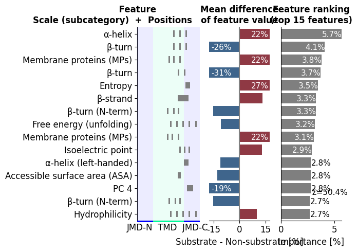
Notice how the top bars are TMD/JMD physicochemical patterns, named
PART-SPLIT-SCALE determinants, not anonymous weights. In the
rendered plot, the left panel shows each feature’s mean_dif (which
way it points: bars to the right sit higher in substrates, bars to the
left higher in non-substrates), while the gray feat_importance bars
on the right show how hard the fitted model leans on each one. Read the
two together: bar height (gray) tells you how much a determinant
matters, and mean_dif direction (left) tells you which way.
Honest evaluation hooks (light). A figure shows what the model leans on; these three quick checks tell you whether it is non-trivial. They are not a substitute for validation:
Cross-validated metrics via
TreeModel.evalover the fitted feature set (fitran withuse_rfe=False, so all features are kept).A trivial baseline, a majority-class
DummyClassifier; a real model must beat its ~0.5 balanced accuracy.Per-protein probabilities via
TreeModel.predict_proba(a mean score and its Monte-Carlo std).
Read these numbers as an optimistic upper bound, not an unbiased
estimate. The CPP signature was mined with labels on the whole
50-protein dataset, then this CV reuses exactly those globally-selected
feature columns, so each fold’s features were chosen using proteins that
also sit in that fold’s test split (feature-selection leakage). It is a
sanity check / ceiling, not a generalization estimate. Leak-free nested
or hold-out evaluation plus shuffled-label controls live in P9:
Validate.
To actually reduce the feature set (recursive feature elimination)
rather than keep all features, fit with
TreeModel(...).fit(X, labels, use_rfe=True) or call
select_features; is_selected_ then marks the retained subset.
# Cross-validated performance of the full fitted feature set (use_rfe=False
# keeps all features; is_selected_ is all-True). Optimistic: the CPP features
# were selected on the full dataset, so this is an upper bound, not a clean
# generalization estimate (see Protocol 9 for leak-free validation).
df_eval = tm.eval(X,
                  labels=labels,
                  list_is_selected=[tm.is_selected_],
                  list_metrics=["accuracy", "balanced_accuracy", "f1", "roc_auc"],
                  n_cv=5)

# Trivial majority-class baseline for comparison (~0.5 balanced accuracy).
from sklearn.dummy import DummyClassifier
from sklearn.model_selection import cross_val_score

baseline_bacc = cross_val_score(
    DummyClassifier(strategy="most_frequent"),
    X, labels, cv=5, scoring="balanced_accuracy").mean()

aa.display_df(df=df_eval.assign(baseline_balanced_accuracy=round(float(baseline_bacc), 3)))
| name | accuracy | balanced_accuracy | f1 | roc_auc | baseline_balanced_accuracy | |
|---|---|---|---|---|---|---|
| 1 | Set 1 | 0.920000 | 0.920000 | 0.925300 | 0.984000 | 0.500000 |
# Per-protein predicted probability of being a substrate (requires prior fit).
import pandas as pd

pred, pred_std = tm.predict_proba(X)
df_pred = pd.DataFrame({
    "entry": df_seq["entry"].to_list(),
    "label": labels,
    "p_substrate": pred.round(3),
    "p_std": pred_std.round(3),
})
# These are IN-SAMPLE (training) predictions, shown only to demonstrate the
# output shape -- they say nothing about generalization. p_std is the spread
# across the ensemble (all tree models over all rounds), i.e. agreement, NOT
# held-out confidence: a small p_std means the models concur, not that the call
# is correct on unseen data. Score real, unseen proteins to judge generalization
# (see Protocol 9).
aa.display_df(df=df_pred.sort_values("p_substrate", ascending=False), n_rows=5)
| entry | label | p_substrate | p_std | |
|---|---|---|---|---|
| 34 | P19022 | 1 | 1.000000 | 0.000000 |
| 30 | Q06481 | 1 | 1.000000 | 0.000000 |
| 44 | Q9ERC8 | 1 | 1.000000 | 0.000000 |
| 33 | P09803 | 1 | 1.000000 | 0.000000 |
| 36 | P09603 | 1 | 1.000000 | 0.000000 |
How to interpret.
Output |
Non-expert reading |
|---|---|
|
the selected TMD/JMD physicochemistry is plausibly discriminative, confirm with leak-free validation in P9: Validate (this light CV is an optimistic upper bound) |
high |
the model ranks substrates above non-substrates reliably |
high |
the determinant the model leans on most for the call |
sign of |
direction of the effect (positive = property higher in substrates) |
|
a substrate (or non-substrate) call; in-sample here, so judge confidence only on unseen proteins |
large |
an unstable prediction (the ensemble models disagree) |
feat_importance is unsigned (magnitude of influence only).
Always pair it with mean_dif from the CPP signature to recover
the biological direction, e.g. higher side-chain volume in the TMD
core rather than just side-chain volume matters.
Key takeaways
The classifier is a glass box: each input is a named
PART-SPLIT-SCALEdeterminant, so a tallfeat_importancebar points at a concrete physicochemical property at a concrete sequence location, read with the sign ofmean_diffor direction.A model is only worth interpreting once it clearly beats the ~0.5 baseline; here balanced accuracy sits well above it.
These numbers are an optimistic ceiling (feature-selection leakage), so treat the result as “plausibly discriminative” and defer real trust to P9: Validate.
Common mistakes.
``CPP(df_seq=…)`` / ``CPP().run(df_seq, labels)``:
CPPtakesdf_parts; build them withSequenceFeature.get_df_partsfirst.Skipping the feature matrix:
TreeModel.fitneeds numericXfromSequenceFeature.feature_matrix, notdf_featordf_seq.Reading ``feat_importance`` as signed: it is magnitude only; combine with
mean_diffor direction.Calling ``predict_proba`` or ``add_feat_importance`` before ``fit``: both rely on attributes set during
.fit.Mistaking light eval for validation: the CV row and baseline here are sanity checks; rigorous trust-building is P9: Validate.
Mis-using ``dPULearn``: it expects labels 1 (positive) and 2 (unlabelled), not 0/1, and
n_unl_to_negmust be >= 1 and must not exceed the number of unlabelled samples.
PU note: when confirmed negatives are scarce. Real GSEC datasets often have confirmed substrates (positives, label 1) but few confirmed non-substrates; the rest are unlabelled (label 2). You cannot train a clean binary classifier on positives-plus-unlabelled directly.
dPULearn (core, no pro dependency) solves the first half: from the
unlabelled pool it identifies reliable negatives (label 0), the
proteins most dissimilar from the positives in CPP feature space, which
you can then feed to the classifier above. See the dPULearn tutorial for
the method details.
Because CPP feature identifiers are dataset-independent strings, the
same df_feat["feature"] builds the feature matrix for the PU
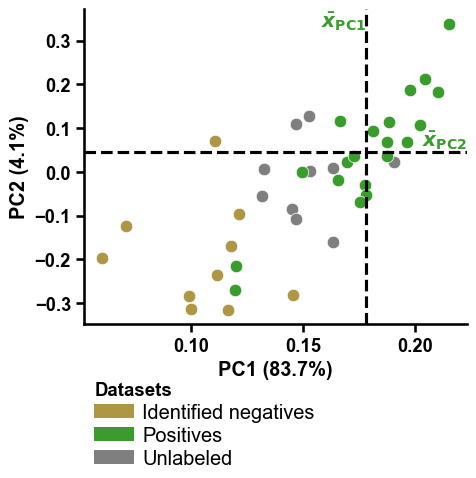
proteins. We demonstrate on the bundled DOM_GSEC_PU dataset, then
visualize the carve with the canonical dPULearn PCA: positives, the
newly carved reliable negatives, and the still-unlabelled pool laid out
in the first two principal components of CPP feature space.
# Positives (1) + unlabelled (2): n=20 -> 20 positives and 20 unlabelled.
df_seq_pu = aa.load_dataset(name="DOM_GSEC_PU", n=20)
labels_pu = df_seq_pu["label"].to_list()

# Reuse the SAME CPP feature ids to build X for the PU proteins.
df_parts_pu = sf.get_df_parts(df_seq=df_seq_pu)
X_pu = sf.feature_matrix(features=df_feat["feature"], df_parts=df_parts_pu, n_jobs=1)

# Carve reliable negatives (0) from the unlabelled pool (2).
# n_unl_to_neg must be >= 1 and must not exceed the number of unlabelled samples (<= 20 here).
# n_components=5 keeps several leading PCs so the carve is visualizable as a PC1-vs-PC2 PCA.
dpul = aa.dPULearn(verbose=False, random_state=42)
dpul = dpul.fit(X=X_pu, labels=labels_pu, n_unl_to_neg=10, n_components=5)

# labels_: 1 = positive, 0 = newly identified reliable negative, 2 = still unlabelled.
import collections
collections.Counter(dpul.labels_.tolist())
Counter({1: 20, 2: 10, 0: 10})
# Headline figure: the dPULearn PCA. The PU proteins are projected into the
# first two principal components of CPP feature space. Dashed lines mark the
# positive-class mean per PC; the unlabelled points (2) furthest from it are
# carved as reliable negatives (0), which then feed the classifier above.
df_pu = dpul.df_pu_
labels_carved = dpul.labels_

aa.plot_settings(font_scale=0.8)
aa.dPULearnPlot().pca(df_pu=df_pu, labels=labels_carved)
plt.tight_layout()
plt.show()
Next step. To explain a single prediction down to per-sample,
single-residue contributions (ShapModel, sample-level
CPPPlot.feature_map), continue to P9: Interpretability.