P6: Compositional vs positional

This protocol contrasts compositional and positional CPP strategies. Once you have two labelled sets of sequences, a test group (label=1) and a reference group (label=0), and you want CPP to tell you what physicochemically distinguishes them, there is one design choice that quietly governs everything: how finely should each feature be localized? A CPP feature is always a Part-Split-Scale triple, and it is the split that decides whether a scale is averaged over a whole part (composition-like, position-agnostic) or over specific sub-regions / positions (location-resolved). You never set a strategy= switch: the strategy emerges from the split_kws recipe you hand to CPP.

This protocol is a determinant-discovery workflow: we contrast two groups and read out the signature of the test group, but here the focus is the shape of that signature. We show how to write each recipe deliberately and how the choice maps onto the prediction level.

Key mental model. Composition answers “what” (how much of a property is present across a part), position answers “where” (at which residues the property differs). Compositional CPP = a single whole-part average, Segment(1,1); positional CPP = sub-segments (n_split_max>1) plus Pattern / PeriodicPattern. As a rule of thumb: compositional ~ protein level (SEQ_*), positional ~ residue level (AA_*), and domain level (DOM_*) happily uses both.

When to use it. Use this protocol when you already have two labelled sets of sequences and need to decide how finely your CPP features should be localized before you commit to a signature. The unit of comparison stays fixed by your prediction level: it is only the locality of the split that you are tuning here.

Question	Strategy	Prediction level
“Is one group globally enriched in a property?” (e.g. whole-chain composition)	Compositional	protein level (SEQ_*)
“Where along the region does the property differ?” (e.g. a residue near a cleavage site)	Positional	residue level (AA_*)
“Both: coarse composition **and* a location-specific signal in a defined sub-region”*	Both	domain level (DOM_*)

Compositional features are coarse and robust (few features, composition-like); positional features are fine and mechanistically actionable but more numerous. The strategy should match the biological resolution your question needs.

When not to use it. If you have not yet built df_parts or chosen a prediction level, start with P1: CPP signature (and the parts/splits engineering in P4: Engineer features) first; this protocol assumes those are settled. It is also not a feature-selection step: here we only shape the split grid; trimming the resulting signature down to a compact, non-redundant set is the job of P7: Select & reduce features (see Next step). And if your question genuinely is global (“is the whole chain enriched?”), do not reach for a dense Pattern / PeriodicPattern grid; that only inflates the feature count without adding interpretive value.

Input. A df_seq with one row per protein and a binary label column, the test group (label=1) versus the reference group (label=0). It comes from an upstream dataset / sampling step (see P1: CPP signature).

Here we work at the domain level with the bundled ``DOM_GSEC`` gamma-secretase dataset, so the unit of comparison is the transmembrane-domain (TMD) part set, native ground for CPP. With n=50 we load 2N = 100 rows (50 substrates + 50 non-substrates). Each row carries entry, sequence, label, and the domain-coordinate columns tmd_start, tmd_stop, jmd_n, tmd, jmd_c that SequenceFeature.get_df_parts consumes.

import aaanalysis as aa

aa.options["verbose"] = False
aa.options["random_state"] = 42

# Two labelled sets of sequences (label: 1 = substrate/test, 0 = reference)
# n=50 -> 2N=100 rows (50 substrates + 50 non-substrates)
df_seq = aa.load_dataset(name="DOM_GSEC", n=50)
labels = df_seq["label"].to_list()
aa.display_df(df=df_seq, n_rows=5)

	entry	sequence	label	tmd_start	tmd_stop	jmd_n	tmd	jmd_c
1	Q14802	MQKVTLGLLVFLAGF...PGETPPLITPGSAQS	0	37	59	NSPFYYDWHS	LQVGGLICAGVLCAMGIIIVMSA	KCKCKFGQKS
2	Q86UE4	MAARSWQDELAQQAE...SPKQIKKKKKARRET	0	50	72	LGLEPKRYPG	WVILVGTGALGLLLLFLLGYGWA	AACAGARKKR
3	Q969W9	MHRLMGVNSTAAAAA...AIWSKEKDKQKGHPL	0	41	63	FQSMEITELE	FVQIIIIVVVMMVMVVVITCLLS	HYKLSARSFI
4	P53801	MAPGVARGPTPYWRL...GLFKEENPYARFENN	0	97	119	RWGVCWVNFE	ALIITMSVVGGTLLLGIAICCCC	CCRRKRSRKP
5	Q8IUW5	MAPRALPGSAVLAAA...EVPATPVKRERSGTE	0	59	81	NDTGNGHPEY	IAYALVPVFFIMGLFGVLICHLL	KKKGYRCTTE

Run. The real entry point is CPP(df_parts=..., split_kws=...).run(labels=...). CPP does not take df_seq / labels directly: you first build sequence parts with SequenceFeature.get_df_parts, then pass a split_kws recipe that encodes the strategy (see the CPP tutorial for the function details). The only thing that differs between compositional and positional is split_kws; the parts are identical.

# Build sequence parts once, shared by both strategies (TMD / JMD-N / JMD-C + composites)
sf = aa.SequenceFeature()
df_parts = sf.get_df_parts(df_seq=df_seq)
aa.display_df(df=df_parts, n_rows=5)

	tmd	jmd_n_tmd_n	tmd_c_jmd_c
entry
Q14802	LQVGGLICAGVLCAMGIIIVMSA	NSPFYYDWHSLQVGGLICAGVL	CAMGIIIVMSAKCKCKFGQKS
Q86UE4	WVILVGTGALGLLLLFLLGYGWA	LGLEPKRYPGWVILVGTGALGL	LLLFLLGYGWAAACAGARKKR
Q969W9	FVQIIIIVVVMMVMVVVITCLLS	FQSMEITELEFVQIIIIVVVMM	VMVVVITCLLSHYKLSARSFI
P53801	ALIITMSVVGGTLLLGIAICCCC	RWGVCWVNFEALIITMSVVGGT	LLLGIAICCCCCCRRKRSRKP
Q8IUW5	IAYALVPVFFIMGLFGVLICHLL	NDTGNGHPEYIAYALVPVFFIM	GLFGVLICHLLKKKGYRCTTE

# --- Recipe A: COMPOSITIONAL (position-agnostic, whole-part average) ---
# A single Segment(1,1) per part -> the feature is a composition-like mean over the ENTIRE part.
split_kws_comp = sf.get_split_kws(split_types="Segment",
                                  n_split_min=1,
                                  n_split_max=1)
split_kws_comp

{'Segment': {'n_split_min': 1, 'n_split_max': 1}}

cpp_comp = aa.CPP(df_parts=df_parts, split_kws=split_kws_comp)
df_feat_comp = cpp_comp.run(labels=labels, n_filter=20)  # compositional yields fewer candidates than positional
aa.display_df(df=df_feat_comp[["feature", "category", "subcategory", "abs_auc", "mean_dif", "positions"]], n_rows=10)

	feature	category	subcategory	abs_auc	mean_dif	positions
1	TMD_C_JMD_C-Seg...1,1)-WOLS870103	Others	PC 4	0.393000	-0.079000	21,22,23,24,25,...,36,37,38,39,40
2	TMD_C_JMD_C-Seg...1,1)-ZIMJ680104	Energy	Isoelectric point	0.339000	0.056000	21,22,23,24,25,...,36,37,38,39,40
3	TMD_C_JMD_C-Seg...1,1)-AURR980112	Conformation	α-helix	0.335000	0.069000	21,22,23,24,25,...,36,37,38,39,40
4	TMD_C_JMD_C-Seg...1,1)-WILM950103	Polarity	Hydrophobicity (interface)	0.288000	-0.059000	21,22,23,24,25,...,36,37,38,39,40
5	TMD_C_JMD_C-Seg...1,1)-GEOR030108	Structure-Activity	Stability (helix-coil)	0.287000	0.076000	21,22,23,24,25,...,36,37,38,39,40
6	TMD_C_JMD_C-Seg...1,1)-CHOP780212	Conformation	β-sheet (C-term)	0.282000	-0.067000	21,22,23,24,25,...,36,37,38,39,40
7	TMD_C_JMD_C-Seg...1,1)-JACR890101	Polarity	Hydrophobicity (surrounding)	0.281000	-0.057000	21,22,23,24,25,...,36,37,38,39,40
8	TMD_C_JMD_C-Seg...1,1)-JANJ780101	ASA/Volume	Accessible surface area (ASA)	0.278000	0.058000	21,22,23,24,25,...,36,37,38,39,40
9	TMD_C_JMD_C-Seg...1,1)-FUKS010109	Composition	AA composition	0.277000	0.061000	21,22,23,24,25,...,36,37,38,39,40
10	JMD_N_TMD_N-Seg...1,1)-KARP850101	Structure-Activity	Flexibility	0.270000	0.057000	1,2,3,4,5,6,7,8...,16,17,18,19,20

# --- Recipe B: POSITIONAL (location-resolved sub-regions / positions) ---
# Sub-segments (n_split_max>1) PLUS Pattern and PeriodicPattern -> features resolve to WHERE in the part.
split_kws_pos = sf.get_split_kws(split_types=["Segment", "Pattern", "PeriodicPattern"],
                                 n_split_min=1,
                                 n_split_max=5,
                                 steps_pattern=[3, 4],
                                 steps_periodicpattern=[3, 4])
split_kws_pos

{'Segment': {'n_split_min': 1, 'n_split_max': 5},
 'Pattern': {'steps': [3, 4], 'n_min': 2, 'n_max': 4, 'len_max': 15},
 'PeriodicPattern': {'steps': [3, 4]}}

cpp_pos = aa.CPP(df_parts=df_parts, split_kws=split_kws_pos)
df_feat_pos = cpp_pos.run(labels=labels, n_filter=30)
aa.display_df(df=df_feat_pos[["feature", "category", "subcategory", "abs_auc", "mean_dif", "positions"]], n_rows=10)

	feature	category	subcategory	abs_auc	mean_dif	positions
1	TMD_C_JMD_C-Seg...2,3)-QIAN880106	Conformation	α-helix	0.387000	0.121000	27,28,29,30,31,32,33
2	TMD_C_JMD_C-Pat...,12)-ROBB760109	Conformation	β-turn (N-term)	0.377000	-0.127000	21,25,28,32
3	TMD_C_JMD_C-Seg...4,5)-ZIMJ680104	Energy	Isoelectric point	0.373000	0.220000	33,34,35,36
4	TMD_C_JMD_C-Seg...4,5)-WOLS870103	Others	PC 4	0.370000	-0.218000	33,34,35,36
5	TMD_C_JMD_C-Seg...3,4)-FAUJ880104	Shape	Side chain length	0.366000	0.205000	31,32,33,34,35
6	TMD_C_JMD_C-Seg...2,3)-WOLS870103	Others	PC 4	0.365000	-0.154000	27,28,29,30,31,32,33
7	TMD_C_JMD_C-Seg...4,5)-ONEK900101	Others	Unclassified (Others)	0.364000	0.097000	33,34,35,36
8	TMD_C_JMD_C-Seg...4,5)-FINA910103	Conformation	α-helix (C-cap)	0.362000	0.264000	33,34,35,36
9	TMD_C_JMD_C-Pat...,15)-QIAN880107	Conformation	α-helix	0.359000	0.158000	25,28,32,35
10	TMD_C_JMD_C-Pat...,15)-MUNV940101	Energy	Free energy (folding)	0.358000	-0.097000	24,28,32,35

# Rank each signature by tree-based feature importance (needed by feature_map).
# One clearly-named TreeModel per strategy keeps the comp/pos blocks parallel.
tm_comp = aa.TreeModel()
X_comp = sf.feature_matrix(features=df_feat_comp["feature"], df_parts=df_parts)
df_feat_comp = tm_comp.fit(X_comp, labels=labels).add_feat_importance(df_feat=df_feat_comp)

tm_pos = aa.TreeModel()
X_pos = sf.feature_matrix(features=df_feat_pos["feature"], df_parts=df_parts)
df_feat_pos = tm_pos.fit(X_pos, labels=labels).add_feat_importance(df_feat=df_feat_pos)

aa.display_df(df=df_feat_pos[["feature", "subcategory", "mean_dif", "abs_auc", "feat_importance"]], n_rows=6)

	feature	subcategory	mean_dif	abs_auc	feat_importance
1	TMD_C_JMD_C-Seg...2,3)-QIAN880106	α-helix	0.121000	0.387000	11.496000
2	TMD_C_JMD_C-Pat...,12)-ROBB760109	β-turn (N-term)	-0.127000	0.377000	6.260000
3	TMD_C_JMD_C-Seg...4,5)-ZIMJ680104	Isoelectric point	0.220000	0.373000	3.071000
4	TMD_C_JMD_C-Seg...4,5)-WOLS870103	PC 4	-0.218000	0.370000	3.670000
5	TMD_C_JMD_C-Seg...3,4)-FAUJ880104	Side chain length	0.205000	0.366000	3.658000
6	TMD_C_JMD_C-Seg...2,3)-WOLS870103	PC 4	-0.154000	0.365000	2.600000

import matplotlib.pyplot as plt
import seaborn as sns

# Feature id is PART-SPLIT-SCALE; the SPLIT field's head names the split type.
def split_type_counts(df_feat):
    types = df_feat["feature"].str.split("-").str[1].str.split("(").str[0]
    return types.value_counts()

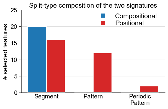
order = ["Segment", "Pattern", "PeriodicPattern"]
counts_comp = split_type_counts(df_feat_comp).reindex(order, fill_value=0)
counts_pos = split_type_counts(df_feat_pos).reindex(order, fill_value=0)

aa.plot_settings(font_scale=0.9, weight_bold=False)
colors = aa.plot_get_clist(n_colors=2)
fig, ax = plt.subplots(figsize=(6, 4))
x = range(len(order))
w = 0.4
ax.bar([i - w / 2 for i in x], counts_comp.values, width=w, label="Compositional",
       color=colors[0], edgecolor="white", zorder=3)
ax.bar([i + w / 2 for i in x], counts_pos.values, width=w, label="Positional",
       color=colors[1], edgecolor="white", zorder=3)
ax.set_xticks(list(x))
ax.set_xticklabels(["Segment", "Pattern", "Periodic\nPattern"])
ax.set_ylabel("# selected features")
ax.set_title("Split-type composition of the two signatures")
ax.set_ylim(0, max(counts_comp.max(), counts_pos.max()) * 1.25)
ax.grid(axis="y", color="0.85", zorder=0)
ax.tick_params(axis="x", length=0)
sns.despine()
aa.plot_legend(dict_color={"Compositional": colors[0], "Positional": colors[1]},
               n_cols=1, x=0.5, y=1.0, marker="s", marker_size=10)
plt.tight_layout()
plt.show()

Output. Both strategies return the same df_feat signature schema (one row per selected feature). Key columns:

• feature: the Part-Split-Scale id (where x how x which property). The Split field is what differs: compositional ids carry only Segment(1,1); positional ids carry Segment(i,n), Pattern(...), or PeriodicPattern(...).

• category / subcategory: the AAontology property group.

• abs_auc: effect size / group-separation strength.

• mean_dif: mean difference (test minus reference); the sign gives the direction.

• positions: the residue positions the feature averages over (a single broad span for compositional; tight, specific positions for positional).

• feat_importance: tree-based importance used to rank the signature.

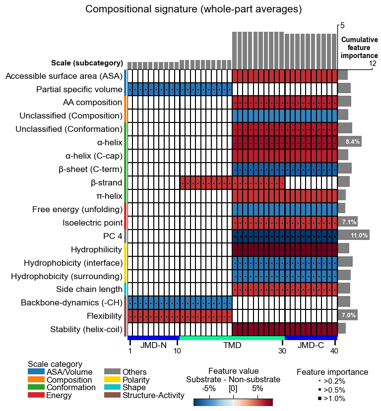
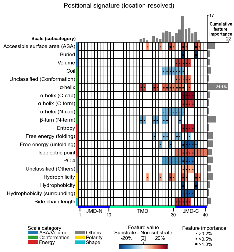
The bar plot above makes the strategic difference concrete: the compositional signature is all ``Segment`` (whole-part means), while the positional signature mixes Segment sub-regions, Pattern, and PeriodicPattern. Read the two feature maps below as rows = properties, columns = positions along the parts, colour = direction x strength.

aa.plot_settings(font_scale=0.7, weight_bold=False)
cpp_plot = aa.CPPPlot()
cpp_plot.feature_map(df_feat=df_feat_comp, name_test="Substrate", name_ref="Non-substrate")
plt.gcf().suptitle("Compositional signature (whole-part averages)", y=1.02)
plt.show()

aa.plot_settings(font_scale=0.7, weight_bold=False)
cpp_plot = aa.CPPPlot()
cpp_plot.feature_map(df_feat=df_feat_pos, name_test="Substrate", name_ref="Non-substrate")
plt.gcf().suptitle("Positional signature (location-resolved)", y=1.02)
plt.show()

How to interpret. Notice how the biological reading mirrors the strategy you chose. The Part- prefix below is schematic: it stands for whichever part actually wins the filter (in this DOM_GSEC run that happens to be the composite TMD_C_JMD_C, as the displayed df_feat shows), so read the ids for their Split field, not the literal part name:

Strategy	Feature id looks like	Biological reading ( gamma-secretase example)	Best prediction level
** Compositional**	...-Seg ment(1,1)-...	“Substrates are richer in small hydrophobic residues across the whole part.”: coarse, co mposition-like, robust.	protein level
Positional	...-Pat tern(...)-... / ...-Seg ment(3,5)-...	“Substrates differ in a charged-residue propensity at specific positions near the cleavage site (TMD centre).”: fine, loc ation-specific, mechanistically actionable.	residue level
Both	mix of the above	domain-level tasks benefit from coarse composition and local position signal in one signature.	domain level

In short: compositional answers “how much” (global property level); positional answers “where” (location of the discriminating property). For mechanism (pinning a signal to a cleavage-adjacent residue), the positional strategy is the more actionable one.

Key takeaways

• The strategy is not a parameter; it emerges from ``split_kws``. Segment(1,1) alone is compositional; adding n_split_max>1 / Pattern / PeriodicPattern makes it positional.

• Both recipes return the same ``df_feat`` signature schema: only the Split field of the feature id (and how tight the positions span is) tells the two apart.

• Match locality to the question: compositional ~ protein level (the “what”), positional ~ residue level (the “where”), domain level uses both.

Common mistakes.

• Using a positional recipe for a protein-level task. Whole-chain composition questions only need Segment(1,1); a large Pattern / PeriodicPattern grid over a long chain explodes the feature count for no interpretive gain.

• Using a compositional recipe for a residue-level task. A single whole-part average cannot localize a site-specific signal, you lose exactly the where the question is about.

• Not matching strategy to prediction level. Remember the mapping: compositional ~ protein, positional ~ residue, domain uses both. There is no strategy= parameter; the strategy emerges from split_kws.

• Forgetting ``feat_importance``. CPPPlot.feature_map is an instance method and needs a feat_importance column; add it with TreeModel.add_feat_importance after fit (skipping this raises in feature_map).

Next step. Both signatures here were capped with a plain n_filter, so they may still carry redundant features. To turn a raw signature into a compact, non-redundant feature set (redundancy reduction plus tree-based feature selection), continue with P7: Select & reduce features.