P2: Exploratory sequence analysis
This is exploratory sequence analysis with no labels: the no-label first look you reach for before you have groups to compare. It sits early in the catalog, right after the CPP signature, before any test-vs-reference contrast exists. When you have sequences but no labels yet, you can still describe what your sequences actually look like before any comparison: the per-position amino-acid composition (a sequence logo) and the per-position conservation (information content, in bits). This is not determinant discovery (CONTEXT.md), the test-vs-reference contrast that yields a signature. There is no contrast here at all: one pooled set, no test/reference split, no signature. We call this no-label first look determinant-free profiling as shorthand throughout (note: “profiling” is our informal label here, not a glossary term).
With no labels you cannot yet ask what distinguishes my groups (that is determinant discovery, see P1: CPP signature). But you can pool every sequence and ask two pre-questions: where along the sequence does signal concentrate, and is there enough structure to make a comparison worth running? A logo answers the first; conservation in bits answers the second.
A one-line decision rule: Do you have labels? No, run exploratory profiling (this protocol). Yes, run CPP signature (P1).
We work at the domain level (dataset prefix DOM_): the unit of
comparison is the TMD-centric part set jmd_n / tmd /
jmd_c, the native ground for CPP.
When to use it. Use this protocol when you have a set of sequences (one biological family, one screen, one organism) and want a first look before committing to any model or comparison. Typical questions:
Is my TMD region more conserved than its flanking JMDs?
Is any single position dominated by one or a few residues?
Are my sequences even structured enough to be worth profiling?
When not to use it. Once you have two labelled sets and want to
know what physicochemically separates them, skip ahead to
determinant discovery via CPP (P1: CPP signature). A logo
describes the composition of one pooled set; it does not contrast
a test group (label=1) against a reference group
(label=0), and it produces no signature.
Input. The input is a df_seq in position-based format: an
entry column (unique protein id), a sequence column, and the
tmd_start / tmd_stop boundaries (1-based, start- and
stop-inclusive).
There is no upstream protocol: this is the no-label first look, used
before you have labels. Its input is whatever sequence table you bring;
here we use a small bundled dataset. Note that a label column may be
present (it is, in DOM_GSEC), but we ignore it on purpose
(profiling is determinant-free).
import matplotlib.pyplot as plt
import aaanalysis as aa

aa.options["verbose"] = False

# DOM_GSEC at the domain level; n=25 per class -> 50 rows. We will NOT use df_seq["label"].
df_seq = aa.load_dataset(name="DOM_GSEC", n=25)
aa.display_df(df=df_seq[["entry", "sequence", "tmd_start", "tmd_stop"]], n_rows=5)
| entry | sequence | tmd_start | tmd_stop | |
|---|---|---|---|---|
| 1 | Q14802 | MQKVTLGLLVFLAGF...PGETPPLITPGSAQS | 37 | 59 |
| 2 | Q86UE4 | MAARSWQDELAQQAE...SPKQIKKKKKARRET | 50 | 72 |
| 3 | Q969W9 | MHRLMGVNSTAAAAA...AIWSKEKDKQKGHPL | 41 | 63 |
| 4 | P53801 | MAPGVARGPTPYWRL...GLFKEENPYARFENN | 97 | 119 |
| 5 | Q8IUW5 | MAPRALPGSAVLAAA...EVPATPVKRERSGTE | 59 | 81 |
# Slice each sequence into the parts we profile.
# Request jmd_n, tmd, jmd_c so the logo spans the full JMD-N + TMD + JMD-C window.
sf = aa.SequenceFeature()
df_parts = sf.get_df_parts(
    df_seq=df_seq,
    list_parts=["jmd_n", "tmd", "jmd_c"],
    jmd_n_len=10,
    jmd_c_len=10,
)
aa.display_df(df=df_parts, n_rows=5)
| jmd_n | tmd | jmd_c | |
|---|---|---|---|
| entry | |||
| Q14802 | NSPFYYDWHS | LQVGGLICAGVLCAMGIIIVMSA | KCKCKFGQKS |
| Q86UE4 | LGLEPKRYPG | WVILVGTGALGLLLLFLLGYGWA | AACAGARKKR |
| Q969W9 | FQSMEITELE | FVQIIIIVVVMMVMVVVITCLLS | HYKLSARSFI |
| P53801 | RWGVCWVNFE | ALIITMSVVGGTLLLGIAICCCC | CCRRKRSRKP |
| Q8IUW5 | NDTGNGHPEY | IAYALVPVFFIMGLFGVLICHLL | KKKGYRCTTE |
Run. Behind the scenes, AALogo aligns the variable-length TMDs
to a fixed width (tmd_len) and tallies the per-position composition
across all sequences (see the AALogo examples for the function
details). We pass no ``labels`` argument, so every sequence is
pooled into a single profile: this is what makes the read-out
determinant-free.
Two quantities come out:
get_df_logo: a composition matrix (probabilityper amino acid, per position).get_df_logo_info: per-position conservation in bits (0 = uniform, ~4.32 = a single fully-conserved residue), whichget_conservationcollapses to a scalar.
Profiling is fully deterministic (every step is a pooled tally), so no
random_state is needed here.
aal = aa.AALogo(logo_type="probability")

# deterministic: pooled tally over all sequences, no RNG -> random_state not applicable.
# tmd_len=20 aligns the variable-length TMDs to a fixed width:
# 10 (jmd_n) + 20 (tmd) + 10 (jmd_c) = 40 positions.
df_logo = aal.get_df_logo(df_parts=df_parts, tmd_len=20)          # (40, 20) pooled composition
df_logo_info = aal.get_df_logo_info(df_parts=df_parts, tmd_len=20)  # per-position bits, index "pos"

cons_mean = aal.get_conservation(df_logo_info=df_logo_info, value_type="mean")
cons_max = aal.get_conservation(df_logo_info=df_logo_info, value_type="max")
cons_mean, cons_max  # returned objects, no print()
(np.float64(1.0053701890712694), np.float64(1.7905267823848006))
Output. Three things flow out: the logo matrix df_logo, the
per-position conservation series df_logo_info, and the scalar
summaries above. The figure below is the single pooled logo: letter
height = composition at that position, and the gray overlay bar =
conservation in bits. Tall, single-letter stacks mark dominated
positions; tall gray bars mark conserved ones.
# Publication styling (plotting_prelude): clean fonts, no bold weight.
aa.plot_settings(font_scale=0.9, weight_bold=False)

aal_plot = aa.AALogoPlot(logo_type="probability", jmd_n_len=10, jmd_c_len=10, verbose=False)
fig, ax = aal_plot.single_logo(
    df_logo=df_logo,
    df_logo_info=df_logo_info,
    figsize=(10, 4),
    fontsize_tmd_jmd=aa.plot_gcfs() + 1,   # legible JMD-N / TMD / JMD-C part labels
    weight_tmd_jmd="bold",
)
plt.show()
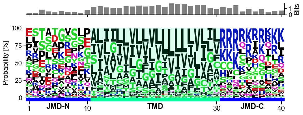
How to interpret. A few things happened here. The colored letters
trace what sits at each position: where the stack collapses onto one
or two tall letters, that position is compositionally dominated. The
gray bars trace how conserved each position is: with a TMD-centric
set like this you will often see the gray bars rise over the
membrane-spanning tmd and stay flatter over the jmd_n /
jmd_c flanks, though on a small pooled set the per-position pattern
can be noisy. That contrast is the whole point: when it appears, it
tells you positional signal concentrates inside the TMD.
Region |
High bits there means … |
|---|---|
|
the juxtamembrane context is constrained, not just variable linker |
|
the membrane span carries a conserved positional pattern, a candidate place to look once you have labels |
Key takeaways
A logo reads composition; information content (bits) reads conservation: two different questions, one figure.
Pooling every sequence is determinant-free: it describes one set, it does not compare groups.
A position with high conservation is a candidate hotspot to revisit once you do have labels and can run a test-vs-reference comparison.
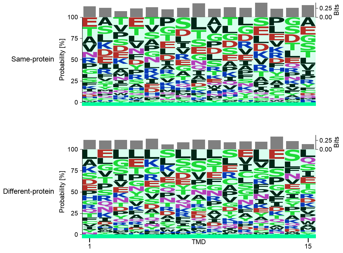
Comparing two groups. The pooled logo above describes one set; it
does not compare groups. To contrast two groups you draw
fixed-length windows per group with AAWindowSampler, then
profile each. Below, sample_same_protein draws TMD-centred windows
from the substrate proteins (Same-protein, the ones carrying a
positive site) and sample_different_protein draws matched windows
from the non-substrate proteins (Different-protein, none). Pooling
each strategy’s equal-length windows into one aligned block and stacking
the two logos with multi_logo() lines them up position by
position, so composition differences read straight off the figure. This
side-by-side is the protocol’s gallery thumbnail, and a preview of P3:
Sampling.
import pandas as pd

# Reproducibility knobs shared with this protocol's gallery thumbnail so both match.
WINDOW_SIZE, N_WINDOWS, SEED = 15, 120, 42

# Mark each substrate's TMD centre as a positive site; leave the non-substrates unlabeled.
# sample_same_protein then draws from proteins that carry a positive site, while
# sample_different_protein draws matched windows from proteins with none.
df_seq_pos = df_seq.copy()
centre = ((df_seq_pos["tmd_start"] + df_seq_pos["tmd_stop"]) // 2).astype(int)
df_seq_pos["pos"] = [[int(c)] if lbl == 1 else [] for c, lbl in zip(centre, df_seq_pos["label"])]

aaws = aa.AAWindowSampler(random_state=SEED)
df_same = aaws.sample_same_protein(df_seq=df_seq_pos, n=N_WINDOWS, window_size=WINDOW_SIZE,
                                   pos_col="pos", seed=SEED)
df_diff = aaws.sample_different_protein(df_seq=df_seq_pos, n=N_WINDOWS, window_size=WINDOW_SIZE,
                                        pos_col="pos", seed=SEED)

# Each strategy's windows are equal-length segments, so pool them into one aligned
# block and profile with AALogo (reusing aal, the probability logo from above).
list_df_logo, list_df_logo_info = [], []
for df_group in (df_same, df_diff):
    df_win = pd.DataFrame({"tmd": df_group["window"].to_list()})
    list_df_logo.append(aal.get_df_logo(df_parts=df_win, tmd_len=WINDOW_SIZE))
    list_df_logo_info.append(aal.get_df_logo_info(df_parts=df_win, tmd_len=WINDOW_SIZE))

# jmd_n_len = jmd_c_len = 0: each pooled window is one aligned block (no JMD flanks).
aal_plot = aa.AALogoPlot(logo_type="probability", jmd_n_len=0, jmd_c_len=0, verbose=False)
fig, ax = aal_plot.multi_logo(
    list_df_logo=list_df_logo,
    list_df_logo_info=list_df_logo_info,
    list_name_data=["Same-protein", "Different-protein"],
    name_data_pos="left",
    figsize_per_logo=(10, 5),
)
plt.tight_layout()
plt.show()
Common mistakes.
Feeding the default parts to the logo plot.
get_df_parts()defaults totmd/jmd_n_tmd_n/tmd_c_jmd_c;AALogothen sees only thetmdcolumn and you get a TMD-only logo. Pairing that withAALogoPlot(jmd_n_len=10, jmd_c_len=10)raises a length error (the JMD lengths no longer fit the logo). Always requestlist_parts=["jmd_n", "tmd", "jmd_c"].Keeping the JMD lengths out of sync.
AALogoPlot(jmd_n_len, jmd_c_len)must match thejmd_n_len/jmd_c_lenyou passed toget_df_parts.Reading a logo as a discriminative result. High conservation across the pooled set says nothing about test vs reference, that needs
CPP. The logo is a one-set description, not a contrast.Wrong unit for residue-level data. For windowed / per-residue tasks (
AA_*) you would first sample fixed-length windows withAAWindowSampler, then profile those: same look-before-you-label idea, different unit of comparison (a window instead of a part set).
Next step. Continue with P3: Sampling to draw the balanced, fixed-length sequence sets you will need once you attach labels and run a comparison.