P4: Prediction levels
This protocol covers the three prediction tasks and levels (residue,
domain, protein) and how each one shapes df_parts. Before you can
ask CPP which physicochemical features separate your groups, you first
have to decide what one example is. Is it a single residue (a
cleavage site, a post-translational modification), one sub-region of a
protein (a transmembrane domain), or a whole chain (a short peptide)?
That choice is the prediction level, and in AAanalysis it is written
directly into the load_dataset() name prefix: AA_* (residue),
DOM_* (domain), SEQ_* (protein). The level is not a different
algorithm: all three feed the same run(). What changes is the
unit of comparison, and therefore how you build df_parts.
Choosing the prediction level fixes the unit of comparison (a
window at residue level, a part set at domain level, or the
whole chain at protein level), and that, in turn, fixes how the
parts are named and which kind of feature you can read out. Pick the
level from your biological question first; the df_parts construction
then follows mechanically.
Like Protocol 1, this is a determinant-discovery / prediction setup: you
contrast a test group (label=1) against a reference group
(label=0) and read out the signature, the set of
position-resolved physicochemical features that separates them. Getting
df_parts right is the single most common bottleneck for new users,
so this protocol shows the correct construction side by side for all
three levels.
When to use it. Use this protocol when you have a labelled two-group
task and are unsure whether it is residue, domain, or
protein level (or when you are building df_parts for the first
time and want a correct template per level). The level follows the
biological question:
Residue level (
AA_*): “What distinguishes a position from its neighbours?” The unit of comparison is a fixed-length window anchored at a residue or a scissile bond (e.g. protease cleavage, PTM sites).Domain level (
DOM_*): “What distinguishes one sub-region of a protein from the same region in another protein?” The unit is a part set derived fromtmd_start/tmd_stop(e.g. gamma-secretase substrates compared over their transmembrane domain), CPP’s native ground.Protein level (
SEQ_*): “What distinguishes one whole chain from another?” The unit is the whole sequence as a single part (e.g. aggregation-prone vs. soluble peptides).
When not to use it. This protocol is about choosing a level and
wiring df_parts: it is not where you sample a reference group. If
your residue-level task has no ready-made negatives (true for most
protease / PTM problems), you must first construct non-site windows; see
the Next step. And if you have only one group, or want to redesign a
sequence rather than contrast two sets, you are outside the
determinant-discovery setup this protocol assumes.
Input. A df_seq whose format matches the level (see
get_df_parts()), plus a binary label column (1
= test group, 0 = reference group). Remember that
load_dataset(name=..., n=N) returns 2N rows (N per group); read
group sizes from the label column, never from len(df_seq). The
level is encoded in the dataset name prefix (AA_* / DOM_* /
SEQ_*; see the data-loader tutorial for the full naming scheme).
Level |
Dataset |
|
Biological contrast (test=1 vs reference=0) |
|---|---|---|---|
residue |
|
s equence-based (9-residue windows around the scissile bond; even window = be tween-residues) |
cleaved ( |
domain |
|
p
osition-based
( |
gamma-secretase
substrate
( |
protein |
|
s equence-based (short full peptides) |
ag
gregation-prone
( |
These tables come from upstream. Domain- and protein-level tables are
loaded directly with load_dataset() (or your own annotation), while
residue-level windows are produced by the Construct sets & sampling
protocol (AAWindowSampler), which is also where you build the
reference group when no negatives exist.
import aaanalysis as aa

aa.options["verbose"] = False
aa.options["random_state"] = 42

sf = aa.SequenceFeature()
Run. The pipeline is identical at every level (get_df_parts ->
run() -> TreeModel ranking), and only df_parts (and the
matching split_kws) differ. We build the three df_parts first,
then run CPP on each.
Residue level: a window as a single part. The 9-residue window is
the unit of comparison, so we map the whole window onto one part. We
set jmd_n_len=0 / jmd_c_len=0 so no flanking is split off, and
select the single neutral part tmd, here just a placeholder name for
“the window”, not a transmembrane domain. (At the residue level the
principled naming follows the Schechter-Berger
... P2 . P1 | P1' . P2' ... convention around the scissile bond;
today parts are chosen from the predefined family, so we keep the
neutral tmd.)
df_res = aa.load_dataset(name="AA_CASPASE3", n=15)
labels_res = df_res["label"].to_list()

df_parts_res = sf.get_df_parts(df_seq=df_res, list_parts=["tmd"], jmd_n_len=0, jmd_c_len=0)
aa.display_df(df=df_parts_res, n_rows=5)
| tmd | |
|---|---|
| entry | |
| CASPASE3_1_pos126 | QTLRDSMLK |
| CASPASE3_1_pos127 | TLRDSMLKY |
| CASPASE3_2_pos116 | VDETDSGAG |
| CASPASE3_2_pos117 | DETDSGAGL |
| CASPASE3_2_pos223 | VDAVDTGIS |
Domain level: named parts from ``tmd_start`` / ``tmd_stop``. The
position-based format lets get_df_parts slice each sequence into the
named parts jmd_n / tmd / jmd_c (here the TMD is the
domain of interest). jmd_n_len / jmd_c_len set how many flanking
residues frame the domain.
df_dom = aa.load_dataset(name="DOM_GSEC", n=15)
labels_dom = df_dom["label"].to_list()

df_parts_dom = sf.get_df_parts(df_seq=df_dom, list_parts=["jmd_n", "tmd", "jmd_c"],
                               jmd_n_len=10, jmd_c_len=10)
aa.display_df(df=df_parts_dom, n_rows=5)
| jmd_n | tmd | jmd_c | |
|---|---|---|---|
| entry | |||
| Q14802 | NSPFYYDWHS | LQVGGLICAGVLCAMGIIIVMSA | KCKCKFGQKS |
| Q86UE4 | LGLEPKRYPG | WVILVGTGALGLLLLFLLGYGWA | AACAGARKKR |
| Q969W9 | FQSMEITELE | FVQIIIIVVVMMVMVVVITCLLS | HYKLSARSFI |
| P53801 | RWGVCWVNFE | ALIITMSVVGGTLLLGIAICCCC | CCRRKRSRKP |
| Q8IUW5 | NDTGNGHPEY | IAYALVPVFFIMGLFGVLICHLL | KKKGYRCTTE |
Protein level: the whole chain as a single part. For whole-chain
prediction the entire sequence is the part. As at the residue level we
set jmd_n_len=0 / jmd_c_len=0 and select the single neutral part
tmd, but here it spans the full peptide, not a window.
df_prot = aa.load_dataset(name="SEQ_AMYLO", n=15)
labels_prot = df_prot["label"].to_list()

df_parts_prot = sf.get_df_parts(df_seq=df_prot, list_parts=["tmd"], jmd_n_len=0, jmd_c_len=0)
aa.display_df(df=df_parts_prot, n_rows=5)
| tmd | |
|---|---|
| entry | |
| AMYLO_1 | AAAQAA |
| AMYLO_2 | QSSYSS |
| AMYLO_3 | QSYGQQ |
| AMYLO_4 | QSYNPP |
| AMYLO_5 | QSYSGY |
Run CPP per level. split_kws must fit the part lengths
(segments/patterns cannot exceed the shortest part). For the short
residue window we use small positional splits; for the domain we
size splits to the 10-residue JMDs; for the protein we use a single
compositional Segment(1,1) whole-part average
(position-agnostic, composition-like).
Notice how the only thing that changes between the three runs is
df_parts (and the split_kws sized to it): the run() ->
TreeModel half is copy-paste identical at every level. To keep the
focus on the figure we show only the domain-level df_feat here, and
visualise that same signature as a feature map in the Output
section just below.
# Residue level: positional splits over the short window
split_kws_res = sf.get_split_kws(split_types=["Segment", "Pattern"], n_split_min=1,
                                 n_split_max=4, steps_pattern=[1, 2], n_min=2, n_max=3, len_max=9)
cpp = aa.CPP(df_parts=df_parts_res, split_kws=split_kws_res)
df_feat_res = cpp.run(labels=labels_res, n_filter=20, n_jobs=1)  # n_jobs=1 avoids a spawn issue on Python 3.14/macOS

X_res = sf.feature_matrix(features=df_feat_res["feature"], df_parts=df_parts_res)
tm = aa.TreeModel().fit(X_res, labels=labels_res)
df_feat_res = tm.add_feat_importance(df_feat=df_feat_res)
# Domain level: splits sized to the named parts (positional + compositional)
split_kws_dom = sf.get_split_kws(n_split_min=1, n_split_max=10, steps_pattern=[3, 4],
                                 n_min=2, n_max=4, len_max=10)
cpp = aa.CPP(df_parts=df_parts_dom, split_kws=split_kws_dom)
df_feat_dom = cpp.run(labels=labels_dom, n_filter=20, n_jobs=1)  # n_jobs=1 avoids a spawn issue on Python 3.14/macOS

X_dom = sf.feature_matrix(features=df_feat_dom["feature"], df_parts=df_parts_dom)
tm = aa.TreeModel().fit(X_dom, labels=labels_dom)
df_feat_dom = tm.add_feat_importance(df_feat=df_feat_dom)
aa.display_df(df=df_feat_dom[["feature", "mean_dif", "abs_auc", "feat_importance"]], n_rows=5)
| feature | mean_dif | abs_auc | feat_importance | |
|---|---|---|---|---|
| 1 | TMD-Pattern(C,4,8)-ROBB760103 | 0.176000 | 0.467000 | 8.380000 |
| 2 | TMD-Pattern(C,4,8)-MUNV940101 | -0.134000 | 0.456000 | 6.685000 |
| 3 | TMD-Pattern(C,4,8)-RACS820114 | -0.191000 | 0.440000 | 6.238000 |
| 4 | TMD-Pattern(C,4,8)-RACS820113 | -0.262000 | 0.436000 | 4.690000 |
| 5 | TMD-Pattern(C,4,8)-NAGK730103 | -0.282000 | 0.431000 | 5.885000 |
# Protein level: compositional Segment(1,1) over the whole chain
split_kws_prot = sf.get_split_kws(split_types="Segment", n_split_min=1, n_split_max=1)
cpp = aa.CPP(df_parts=df_parts_prot, split_kws=split_kws_prot)
df_feat_prot = cpp.run(labels=labels_prot, n_filter=15, n_jobs=1)  # n_jobs=1 avoids a spawn issue on Python 3.14/macOS

X_prot = sf.feature_matrix(features=df_feat_prot["feature"], df_parts=df_parts_prot)
tm = aa.TreeModel().fit(X_prot, labels=labels_prot)
df_feat_prot = tm.add_feat_importance(df_feat=df_feat_prot)
Output. Each level returns its own df_feat signature, one
row per selected feature, with the feature id reading as
Part-Split-Scale. The downstream columns are identical across
levels: mean_dif (signed test minus reference difference),
abs_auc (separation strength, the adjusted AUC* in [0, 0.5]
where 0 = no separation and 0.5 = perfect separation), and
feat_importance (tree-based rank). The only thing that changes is
how the feature id reads, because the parts differ; everything
downstream stays the same.
A note on the numbers. We deliberately use tiny
n=15-per-group fixtures so the protocol runs in seconds. On so few sequences it is trivial for top-ranked features to separate the two groups perfectly, so you will seeabs_aucsitting at or near0.5(especially at the residue level, where the short windows overfit most easily). Treat these values as illustrative of what the column means, not as a real effect size; on a full dataset the same ranking shows a graded spread ofabs_aucbelow0.5.
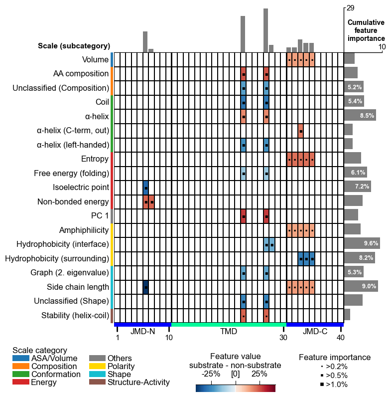
The fastest way to see a signature is the feature map (the same plot
as in Protocol 1). Below is the domain-level (gamma-secretase)
signature: the y-axis groups features by AAontology category, the
heatmap cells show mean_dif (red = higher in substrates, blue =
higher in non-substrates), and the bars on the right show
feat_importance.
import matplotlib.pyplot as plt

aa.plot_settings(font_scale=0.65, weight_bold=False)
cpp_plot = aa.CPPPlot()                 # feature_map is an INSTANCE method
cpp_plot.feature_map(df_feat=df_feat_dom, name_test="substrate", name_ref="non-substrate")
plt.tight_layout()
plt.show()
The feature ids read differently per level because the parts differ:
Level |
|
Example feature |
Reads as |
|---|---|---|---|
residue |
|
|
which positions in the window, which property |
domain |
|
|
which sub-region of the domain, which property |
protein |
|
|
a whole-chain composition property (no position) |
Visualise any level’s signature with
aa.CPPPlot().feature_map(df_feat=...) exactly as above: the plot
needs the feat_importance column we added with
add_feat_importance().
How to interpret. Read each output column as follows:
Output |
Non-expert reading |
|---|---|
|
stronger group-separating
property; |
positive |
property is higher in the test group (label=1) |
negative |
property is higher in the reference group (label=0) |
a |
a compositional signal (it does not depend on position) |
a |
a positional signal (it depends on where in the part) |
The level constrains the kind of feature you can read:
Residue signatures are purely positional: e.g. CASPASE3 cleavage depends on which flanking position (P2, P3, P4 …) carries which property around the scissile bond.
Protein signatures are purely compositional: amyloid aggregation depends on overall composition, not position, so only
Segment(1,1)features appear.Domain signatures mix both: the gamma-secretase TMD shows positional sub-region effects and whole-part composition.
Key takeaways
The prediction level you pick fixes the unit of comparison and how parts are named: it is a modelling decision, not an algorithm switch; all three levels call the same
run().The level constrains the kind of signature: residue is purely positional, protein is purely compositional, domain mixes both.
Always read the signature (coherent blocks of related features), never a single cell, and on tiny fixtures read
abs_aucas illustrative, not as a real effect size.
Common mistakes.
Calling ``CPP(df_seq=…)``:
CPPtakesdf_parts; always build them withget_df_parts()first (true at every level).Forgetting that “part” means different things per level: a window (residue), a named sub-region (domain), or the whole chain (protein). Name and interpret it accordingly.
Using positional splits at the protein level: whole-chain composition is best captured by the compositional
Segment(1,1); multi-segment /Patternsplits over-fragment a position-agnostic signal.Letting ``split_kws`` exceed the shortest part: segments and patterns cannot be longer than the smallest part (e.g. a 10-residue JMD or a 9-residue window), or
CPPraises a “too short sequences” error. Sizen_split_max/len_maxto the parts.Confusing residue with domain: both can use a single
tmdpart, but residue windows are short, fixed-length, and anchored at a site, while domain parts come fromtmd_start/tmd_stopand carry flanking JMDs (jmd_n_len/jmd_c_len).
Next step. Continue with P5: Engineer features to turn the chosen
prediction level and its df_parts into an engineered CPP feature
set.