P5: Engineer features
This protocol engineers the CPP feature space: parts, splits, and
numerical channels (embeddings or structure). Feature engineering is the
stage between raw sequences and a CPP signature. Before Comparative
Physicochemical Profiling (CPP) can contrast a test group
(label=1) against a reference group (label=0) and read out
what physicochemically distinguishes them, every protein has to be
turned into a structured feature space. AAanalysis builds that space
from one small grammar: a feature is always a Part-Split-Scale
triple, a named region (part), a rule for which positions to
average (split), and a value axis. Here we engineer that space at
the domain level (dataset prefix DOM_), where the unit of
comparison is the TMD-centric part set.
A feature = part × split × scale: where in the sequence (tmd,
jmd_n_tmd_n, tmd_c_jmd_c), how the positions are picked
(Segment / Pattern / PeriodicPattern), and what value is
averaged. The value axis has two interchangeable sources: a
physicochemical scale (the sequence arm, run()) or a
per-residue numerical tensor, a protein-language-model (PLM) embedding
or a structure channel (the numerical arm, run_num()). Same
grammar, same df_feat output; only the value source changes. That is
exactly what lets learned and structural representations ride the same
interpretable CPP machinery.
When to use it. Reach for this protocol once you have labelled
sequences (a df_seq with a binary label) and need to turn them
into a CPP-ready feature space, the step that sits underneath every CPP
run, whether the downstream task is determinant discovery or
prediction. It answers the three engineering questions hiding under
that grammar:
Where? Slice each protein into TMD-centric parts. By default
get_df_partsreturns the base parttmdplus the compositesjmd_n_tmd_nandtmd_c_jmd_c(built from the base partsjmd_n/tmd/jmd_c).Which positions? Pick a split type:
Segment(a contiguous block),Pattern, orPeriodicPattern(spaced positions).What value? Average a physicochemical scale (the sequence arm, consumed by
run()) or a per-residue numerical vector such as a PLM embedding or a structural channel (the numerical arm, consumed byrun_num()).
Both arms share the identical Part-Split grammar and emit the identical
df_feat schema, so anything you learn on the sequence arm transfers
directly to embeddings and structure.
When not to use it. Skip the manual enumeration if you just want a
signature with sensible defaults: run() builds parts and splits
internally, so you only need this protocol when you want to control
the feature space or feed in numerical channels. It is also not where
you decide the compositional vs positional trade-off (that is P6:
Compositional vs positional), and for residue-level tasks you first
manufacture fixed-length windows (parts named by the Schechter-Berger
convention) in Protocol 3 - Construct sets & sampling before
engineering features.
Input. A df_seq with one row per protein: an entry
identifier, a sequence, and a binary label (test group = 1
vs. reference group = 0). For a domain-level task it also
carries tmd_start / tmd_stop, from which the part boundaries
are derived. Upstream this df_seq typically arrives from Protocol 3
- Construct sets & sampling (residue level) or from a curated labelled
set (domain level, as here).
The numerical arm adds one more input: a dict_num mapping each
entry to a per-residue tensor of shape (L, D), where L
equals the sequence length and D is the number of numerical channels
(embedding or structure dimensions). Real PLM embeddings (ProtT5, ESM)
are heavy to compute, so you generate them separately on a GPU
(e.g. the companion Colab notebook), then save the (L, D) tensors
and load them here; AAanalysis never runs the model itself. To keep this
protocol offline and fast we instead build a small synthetic
dict_num with NumPy. The real workflow would substitute a ProtT5 /
ESM embedding or a DSSP / structure tensor of the same (L, D) shape.
We use the bundled DOM_GSEC gamma-secretase dataset (substrates
vs. non-substrates) throughout.
import aaanalysis as aa
import numpy as np

aa.options["verbose"] = False
aa.options["random_state"] = 42

# Domain-level gamma-secretase data: substrates (label=1) vs non-substrates (0).
# load_dataset(name=..., n=10) returns 2*n = 20 rows (10 per class).
df_seq = aa.load_dataset(name="DOM_GSEC", n=10)
labels = df_seq["label"].to_list()          # use the label column, NOT len(df_seq)
aa.display_df(df=df_seq, n_rows=5)
| entry | sequence | label | tmd_start | tmd_stop | jmd_n | tmd | jmd_c | |
|---|---|---|---|---|---|---|---|---|
| 1 | Q14802 | MQKVTLGLLVFLAGF...PGETPPLITPGSAQS | 0 | 37 | 59 | NSPFYYDWHS | LQVGGLICAGVLCAMGIIIVMSA | KCKCKFGQKS |
| 2 | Q86UE4 | MAARSWQDELAQQAE...SPKQIKKKKKARRET | 0 | 50 | 72 | LGLEPKRYPG | WVILVGTGALGLLLLFLLGYGWA | AACAGARKKR |
| 3 | Q969W9 | MHRLMGVNSTAAAAA...AIWSKEKDKQKGHPL | 0 | 41 | 63 | FQSMEITELE | FVQIIIIVVVMMVMVVVITCLLS | HYKLSARSFI |
| 4 | P53801 | MAPGVARGPTPYWRL...GLFKEENPYARFENN | 0 | 97 | 119 | RWGVCWVNFE | ALIITMSVVGGTLLLGIAICCCC | CCRRKRSRKP |
| 5 | Q8IUW5 | MAPRALPGSAVLAAA...EVPATPVKRERSGTE | 0 | 59 | 81 | NDTGNGHPEY | IAYALVPVFFIMGLFGVLICHLL | KKKGYRCTTE |
Run: Arm A, sequence features (scale-based). The sequence arm turns
df_seq into a CPP-ready feature space in three small steps: slice
the parts, configure how to split, then enumerate the full grammar
(see the SequenceFeature tutorial, tutorial3b_sequence_feature, for
the function details):
get_df_parts()slices each protein into the TMD-centric parts (by default the base parttmdplus the compositesjmd_n_tmd_nandtmd_c_jmd_c), producing thedf_partsthatCPPconsumes.get_split_kws()builds the split configuration, one entry per split type (Segment,Pattern,PeriodicPattern).get_features()enumerates the fullPart-Split-Scalespace as a list of feature ids.
sf = aa.SequenceFeature()

# 1) Parts: slice sequences into TMD-centric parts
df_parts = sf.get_df_parts(df_seq=df_seq)

# 2) Split configuration: Segment / Pattern / PeriodicPattern
split_kws = sf.get_split_kws()

# Split types in the configuration: ['Segment', 'Pattern', 'PeriodicPattern']
list(split_kws)
['Segment', 'Pattern', 'PeriodicPattern']
# 3) Enumerate the PART-SPLIT-SCALE space. The full scale set explodes
#    combinatorially, so restrict to a 3-scale slice for the demo.
df_scales = aa.load_scales()
small_scales = list(df_scales.columns[:3])

features = sf.get_features(split_kws=split_kws, list_scales=small_scales)
# Number enumerated (3 parts x splits x 3 scales): len(features)
len(features), features[:5]
(2970,
 ['TMD-Segment(1,1)-ANDN920101',
  'TMD-Segment(1,1)-ARGP820101',
  'TMD-Segment(1,1)-ARGP820102',
  'TMD-Segment(1,2)-ANDN920101',
  'TMD-Segment(1,2)-ARGP820101'])
# Optional: reduce redundancy. Build the feature matrix, then drop columns
# that correlate above max_cor with an already-kept feature.
# Note: filter_correlation keeps the FIRST-SEEN representative of each
# correlated group. Applied pre-CPP on the raw PART-SPLIT-SCALE enumeration
# order, it yields a redundancy-reduced but importance-agnostic set. To keep
# the most important representative, apply it to an importance-ordered
# CPP.run / df_feat output instead (see Protocol 1 - CPP signature).
X = sf.feature_matrix(features=features, df_parts=df_parts, n_jobs=1)
is_selected = aa.NumericalFeature.filter_correlation(X, max_cor=0.7)

# Features kept after redundancy filtering:
int(is_selected.sum())
368
Run: Arm B, numerical features (embeddings / structure). The numerical arm replaces the per-AA scale lookup with a per-residue tensor. The Part-Split grammar is unchanged; only the value source differs.
The Arm B tensor below is synthetic NumPy noise, so every ``abs_auc`` / ``mean_dif`` it produces is pure chance: treat it as a plumbing demo, not a signature. Swap in a real ProtT5 / ESM embedding or a DSSP / structure tensor of the same
(L, D)shape for a meaningful readout.
Build a
dict_numof{entry: (L, D) ndarray}. We synthesise one withnp.random.default_rng(42);rng.randomalready yields values in[0, 1), which is exactly the rangerun_num()expects (itsmax_std_testpre-filter is calibrated for[0, 1]), so no normalisation step is needed. With real PLM embeddings the values are unbounded, so you would first run them throughencode()(embp.encode(df_seq=df_seq, embeddings=...), the sanctioned step from raw embeddings todict_numthat fits one[0, 1]normaliser per channel) beforeget_parts.:meth:`~aaanalysis.EmbeddingPreprocessor.build_scales` / ``build_cat`` name the
Ddimensions (df_scalesof shape(20, D),df_catof shape(D, ...)) so theCPPinvariantD == len(df_scales.columns) == len(df_cat)holds. The per-AA scale values are not the per-residue value source forrun_num(that isdict_num_parts), but thedf_catcategories, derived from these pseudo-scales by clustering, do drive category-aware redundancy filtering and grouping. Derivingdf_scales/df_catfrom the samedict_num(rather than fabricating an arbitrary(20, D)/df_cat) is therefore what keeps both the invariant and the categories meaningful.:meth:`~aaanalysis.NumericalFeature.get_parts` slices the sequence strings AND the tensor with the same boundaries, returning
(df_parts, dict_num_parts).:meth:`~aaanalysis.CPP.run_num` runs the identical CPP algorithm on the sliced tensor.
D = 4                                   # tiny embedding dimensionality
rng = np.random.default_rng(42)

# Per-residue tensor: one (L, D) array per entry, L == sequence length, in [0, 1)
dict_num = {e: rng.random((len(s), D))
            for e, s in zip(df_seq["entry"], df_seq["sequence"])}

# Name the D dimensions. dict_num_parts (not these per-AA values) is the
# per-residue value source for run_num; but df_cat's categories - derived
# from these pseudo-scales - drive category-aware redundancy filtering, so we
# derive both from the same dict_num rather than fabricating them.
# Shapes: df_scales_num is (20, D); df_cat_num is (D, ...).
embp = aa.EmbeddingPreprocessor()
df_scales_num = embp.build_scales(df_seq=df_seq, dict_num=dict_num)
df_cat_num = embp.build_cat(df_scales=df_scales_num, random_state=42)
aa.display_df(df=df_scales_num, n_rows=5)
/var/folders/sv/65tlch_10198qgmpwcp6408r0000gn/T/ipykernel_43985/3470844455.py:14: UserWarning: Pseudo-scales are dataset-dependent (averaged over df_seq). For reproducible cross-dataset comparison, compute them once on a fixed reference corpus and reuse the resulting df_scales.
  df_scales_num = ep.build_scales(df_seq=df_seq, dict_num=dict_num)
| dim_0 | dim_1 | dim_2 | dim_3 | |
|---|---|---|---|---|
| A | 0.492584 | 0.497712 | 0.485069 | 0.513540 |
| C | 0.502098 | 0.506278 | 0.518440 | 0.502096 |
| D | 0.487394 | 0.508945 | 0.499097 | 0.498795 |
| E | 0.482504 | 0.494474 | 0.511045 | 0.497436 |
| F | 0.508067 | 0.473032 | 0.475938 | 0.501151 |
# Slice sequences AND tensor with shared part boundaries
df_parts_num, dict_num_parts = aa.NumericalFeature.get_parts(df_seq=df_seq, dict_num=dict_num)

# Each part tensor has shape (n_samples, L_part_max, D), NaN-padded
{k: v.shape for k, v in dict_num_parts.items()}
{'tmd': (20, 23, 4), 'jmd_n_tmd_n': (20, 22, 4), 'tmd_c_jmd_c': (20, 21, 4)}
# Numerical-mode CPP: same algorithm and df_feat schema as CPP.run
cpp = aa.CPP(df_parts=df_parts_num,
             df_scales=df_scales_num,
             df_cat=df_cat_num,
             verbose=False)
df_feat = cpp.run_num(dict_num_parts=dict_num_parts,
                      labels=labels,
                      n_filter=10,
                      n_jobs=1)        # serial: avoids spawn footgun on Py3.14 + macOS
aa.display_df(df=df_feat[["feature", "category", "subcategory", "mean_dif", "abs_auc"]], n_rows=5)
| feature | category | subcategory | mean_dif | abs_auc | |
|---|---|---|---|---|---|
| 1 | TMD_C_JMD_C-Pat...C,4,7,10)-dim_1 | Embeddings | Embeddings_cat1_subcat0 | -0.216000 | 0.360000 |
| 2 | TMD_C_JMD_C-Pat...,9,12,15)-dim_1 | Embeddings | Embeddings_cat1_subcat0 | -0.174000 | 0.360000 |
| 3 | JMD_N_TMD_N-Pat...,6,10,14)-dim_0 | Embeddings | Embeddings_cat0_subcat1 | 0.174000 | 0.360000 |
| 4 | JMD_N_TMD_N-Pat...,8,11,14)-dim_3 | Embeddings | Embeddings_cat0_subcat2 | 0.165000 | 0.350000 |
| 5 | TMD-Pattern(N,2,5,8)-dim_3 | Embeddings | Embeddings_cat0_subcat2 | 0.152000 | 0.340000 |
# Multiple per-residue sources combine along the D axis before get_parts.
# Here a second synthetic channel stands in for a structural tensor.
dict_struct = {e: rng.random((len(s), 2)) for e, s in zip(df_seq["entry"], df_seq["sequence"])}
dict_combined = aa.combine_dict_nums([dict_num, dict_struct])
{e: dict_combined[e].shape for e in list(dict_combined)[:3]}   # D = 4 + 2 = 6
{'Q14802': (87, 6), 'Q86UE4': (582, 6), 'Q969W9': (287, 6)}
Output. Arm A (sequence) produces three objects: - df_parts:
one row per protein, one column per part (tmd, jmd_n_tmd_n,
tmd_c_jmd_c); the primary input to CPP. - split_kws: the
split configuration dict. - features: a list of
Part-Split-Scale feature ids, optionally reduced by
filter_correlation.
Arm B (numerical) produces: - (df_parts_num, dict_num_parts)
from get_parts; each dict_num_parts[part] is a NaN-padded array
of shape (n_samples, L_part_max, D), aligned row-for-row with
df_parts_num. - df_feat: the signature, with the same
schema as run() (feature, category, subcategory,
mean_dif, abs_auc, …). The value axis is now the embedding
channels (dim_0 … dim_3) instead of physicochemical scales.
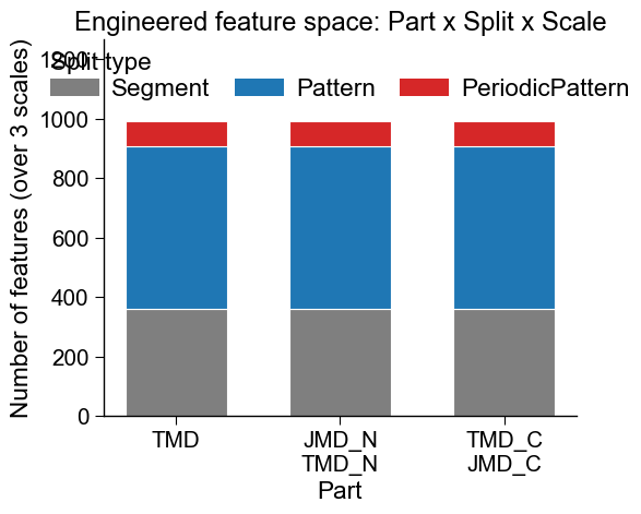
The bar plot below makes the engineered Arm A space concrete: it tallies
the features enumeration by part (x-axis) and split type
(colour). Notice how every part carries the same Segment /
Pattern / PeriodicPattern stack: the grammar is uniform across
parts, and what multiplies the count is simply how many scales (sequence
arm) or numerical channels (numerical arm) you enumerate over.
import matplotlib.pyplot as plt
import seaborn as sns

# Tally the Arm A enumeration: every feature id is a Part-Split-Scale triple,
# so we count features by part (x-axis) and split type (stacked colour).
parts_order = ["TMD", "JMD_N_TMD_N", "TMD_C_JMD_C"]
part_labels = ["TMD", "JMD_N\nTMD_N", "TMD_C\nJMD_C"]
split_types = list(split_kws)                 # ['Segment', 'Pattern', 'PeriodicPattern']
counts = {st: [0] * len(parts_order) for st in split_types}
for feat in features:
    tokens = feat.split("-")
    part, split = tokens[0], tokens[1]
    st = split.split("(")[0]
    if part in parts_order and st in counts:
        counts[st][parts_order.index(part)] += 1

# Publication styling (plotting_prelude): clean stacked bar with despine + tidy legend.
aa.plot_settings(font_scale=0.9, weight_bold=False)
colors = aa.plot_get_clist(n_colors=len(split_types))

fig, ax = plt.subplots(figsize=(6, 5))
x = range(len(parts_order))
bottom = [0] * len(parts_order)
dict_color = {}
for st, color in zip(split_types, colors):
    ax.bar(x, counts[st], bottom=bottom, label=st, color=color,
           width=0.62, edgecolor="white", linewidth=0.8)
    bottom = [b + c for b, c in zip(bottom, counts[st])]
    dict_color[st] = color

total = max(bottom)
ax.set_xticks(list(x))
ax.set_xticklabels(part_labels)
ax.set_ylim(0, total * 1.28)
ax.set_xlabel("Part")
ax.set_ylabel("Number of features (over 3 scales)")
ax.set_title("Engineered feature space: Part x Split x Scale",
             size=aa.plot_gcfs() + 1)
sns.despine()

# Clean horizontal legend in the headroom above the bars (no occlusion).
aa.plot_legend(ax=ax, dict_color=dict_color, title="Split type",
               loc="upper center", x=0.5, y=1.0, n_cols=3,
               columnspacing=1.0, handletextpad=0.5)

plt.tight_layout()
plt.show()
How to interpret.
Output |
Reading |
|---|---|
a |
the default parts (the base part
|
a |
the rule for which positions
are averaged ( |
a |
where + how + which physicochemical property |
a |
where + how + which
embedding / structure channel
( |
|
direction of separation (positive = higher in the test group in that region) |
|
effect size / separation strength of the feature |
Both arms read the same way: a coherent block of high-abs_auc
features from one property family or embedding channel, localized to one
part, is the signature that distinguishes substrates from
non-substrates. The numerical arm simply lets you profile learned /
structural representations with the same interpretable grammar. One
caveat for this demo: because the Arm B tensor is synthetic NumPy noise,
the abs_auc / mean_dif values shown above are not
biologically meaningful (the small effect sizes are pure chance). Swap
in a real ProtT5 / ESM embedding or a DSSP / structure tensor of the
same (L, D) shape and the identical readout surfaces the channels
that actually separate the test group from the reference group.
Key takeaways - A feature is always part × split × scale:
control where, how, and what value independently, and the
engineered space follows mechanically. - The sequence arm
(run(), physicochemical scales) and the numerical arm
(run_num(), per-residue tensors via dict_num) share one
grammar and one df_feat schema, so embeddings and structure ride the
same interpretable machinery. - The shape of the space is yours to set:
enumerate broadly to explore, then reduce redundancy with
filter_correlation before committing to a CPP run.
Common mistakes.
Passing ``df_seq`` into :class:`~aaanalysis.CPP`:
CPPtakesdf_parts; build them withget_df_parts(Arm A) orget_parts(Arm B) first.Feeding raw, unbounded embeddings into ``run_num``: values must be in
[0, 1](themax_std_testpre-filter is calibrated for that range); pass real PLM embeddings throughencode()first. Our synthetic tensor is already in range, so it skips that step.``dict_num`` length mismatch: each
dict_num[entry]must haveL == len(sequence); otherwiseget_partscannot align the tensor to the parts.``D`` mismatch:
Dmust equallen(df_scales.columns)andlen(df_cat); deriving both withbuild_scales/build_catfrom the samedict_numkeeps the invariant.Using ``len(df_seq)`` for class sizes: use the
labelcolumn;load_dataset(..., n=N)returns2Nrows.Relying on the default ``n_jobs``: on Python 3.14 + macOS, multiprocessing spawn without a
__main__guard is fragile; passn_jobs=1in notebooks.Enumerating the full scale set:
get_featuresover hundreds of scales explodes combinatorially; slicelist_scalesfor exploration.
Next step.
Compositional vs positional leads to P6: Compositional vs positional. You now know a feature is
Part-Split-Scale; P6 shows how the split alone decides whether a feature is composition-like (whole-partSegment(1,1), position-agnostic) or position-resolved (Segmentwithn_split_max > 1,Pattern,PeriodicPattern), and how that choice maps onto the prediction level.Run the signature by feeding the engineered
df_partsstraight into the CPP signature: see Protocol 1 - CPP signature.