P3: Sampling
This protocol covers constructing sets and sampling: windows, reference and control. Residue-level questions (where does a protease cut? which residue is modified?) are never asked over a whole protein. They are asked over short, fixed-length windows anchored on candidate sites. And here is the catch that trips up most newcomers: the known positives are only ever a handful of annotated sites, so the reference they must be compared against does not exist yet, you have to build it. How you draw those reference windows quietly decides what any downstream model or CPP signature can possibly learn.
A fair comparison needs fair reference and control windows. The test
group (label=1) is the set of test windows sitting at known
P1 anchors; the reference group (label=0) is the set of
reference windows you sample around them. Draw that reference
unfairly (too easy, too similar, or composition-skewed) and the contrast
measures your sampling, not the biology. AAWindowSampler is the tool
that builds this set reproducibly, with anti-leakage and redundancy
filters baked in.
This protocol is a determinant-discovery / prediction building block
at the residue level, the companion to P1: CPP signature (which
works at the domain level). Here we manufacture the windowed input
that a residue-level CPP run or downstream classifier consumes. For the
mechanics of each sampling method, see the AAWindowSampler examples;
here we focus on the workflow.
When to use it. Use this protocol for residue-level prediction: the biological unit is a single site, scored over a fixed-length window (glossary: residue level). Two sub-modes, distinguished only by window parity:
between-residues (even
window_size): a scissile bond… P2·P1 │ P1′·P2′ …(Schechter–Berger), e.g. protease cleavage, our running caspase-3 example.single-residue (odd
window_size): a site on a residue, e.g. a PTM (phosphorylation, glycosylation).
This is distinct from the domain level (P1: CPP signature,
comparison over jmd_n/tmd/jmd_c parts) and the protein
level (whole-chain). The defining difficulty at the residue level is
reference construction: positives are a handful of annotated sites,
but the negatives must be manufactured, and how you draw them (same
protein, other proteins, or synthetic) changes what the downstream model
learns.
When not to use it. Skip this protocol when your data is already
windowed (one fixed-length slice per row with a binary label):
there is nothing left to sample, so go straight to P4: Prediction
levels. Skip it too for domain-level work (contrast jmd_n /
tmd / jmd_c parts, see P1: CPP signature) and
protein-level work (the whole chain is the unit of comparison),
where no window is sampled.
Input. A df_seq with one row per full protein sequence
(entry + sequence) and a pos column (default name pos):
each cell is a list[int] of 1-based P1 anchors, the known
positive sites on that protein (empty list = no annotated site). This is
the upstream format produced by an annotation step
(e.g. to_df_seq(), or your own curation of
literature cleavage sites).
Note: the bundled
aa.load_dataset(name="AA_CASPASE3")returns sequences that are already windowed (one 9-mer per row, with a binarylabel): it is the output of a sampling step, not the input to one. To demonstrate the sampler we therefore start from full sequences with aposcolumn, which is exactly whatAAWindowSamplerexpects.
Rows that carry positives are substrate proteins; rows with an empty
pos cell are non-substrate proteins, the latter form the
candidate pool for cross-protein sampling.
import aaanalysis as aa
import pandas as pd

aa.options["verbose"] = False
aa.options["random_state"] = 42

# Full-sequence df_seq for caspase-3 cleavage (P1 anchor = the Asp of a D-x-x-D motif).
# Substrate proteins carry 1-based P1 anchors in `pos`; non-substrate proteins have [].
df_seq = pd.DataFrame({
    "entry": ["SUB1", "SUB2", "SUB3", "NEG1", "NEG2", "NEG3"],
    "sequence": [
        "MKTAYIAKQRDEVDSGLAPYKVLNMQATGHIWDETDSARKLMNPQRSTV",
        "GASPMNLKDEVDTAGRWFYHCIKLMNPQRSTVWYDQTDSGKLAANPQRS",
        "MQALDEVDGKLMNPQRSTVWYACDEFGHIKLMNPQRSTVWYAKLM",
        "ACDEFGHIKLMNPQRSTVWYACDEFGHIKLMNPQRSTVWYACDEFGHIK",
        "GHIKLMNPQRSTVWYACDEFGHIKLMNPQRSTVWYGHIKLMNPQRSTVW",
        "WYACDEFGHIKLMNPQRSTVWYKLMNPQRSTVWYACDEFGHIKLMNPQR",
    ],
    "pos": [[14, 36], [9, 35], [9], [], [], []],
})
# `n_pos` = number of annotated P1 anchors (>0 -> substrate, 0 -> non-substrate pool).
aa.display_df(df=df_seq.assign(n_pos=df_seq["pos"].apply(len)), n_rows=6)
| entry | sequence | pos | n_pos | |
|---|---|---|---|---|
| 1 | SUB1 | MKTAYIAKQRDEVDS...TDSARKLMNPQRSTV | [14, 36] | 2 |
| 2 | SUB2 | GASPMNLKDEVDTAG...DQTDSGKLAANPQRS | [9, 35] | 2 |
| 3 | SUB3 | MQALDEVDGKLMNPQ...LMNPQRSTVWYAKLM | [9] | 1 |
| 4 | NEG1 | ACDEFGHIKLMNPQR...RSTVWYACDEFGHIK | [] | 0 |
| 5 | NEG2 | GHIKLMNPQRSTVWY...YGHIKLMNPQRSTVW | [] | 0 |
| 6 | NEG3 | WYACDEFGHIKLMNP...ACDEFGHIKLMNPQR | [] | 0 |
Run. AAWindowSampler exposes four methods, each producing the
same segments-mode schema: sample_same_protein (within-protein
hard negatives), sample_different_protein (cross-protein unlabeled
pool), sample_synthetic (composition controls), and
sample_benchmark_set (a reproducible multi-arm orchestrator). The
cells below demonstrate each in turn, assigning a fitting role to
every sampled window. For per-method parameter details, see the
AAWindowSampler examples (this protocol stays at the workflow
level).
Role vs. strategy. Every sampled window carries two orthogonal tags (glossary):
role (
rolecolumn): the workflow meaning of the row:Test,Negative,Unlabeled, orControl. It answers “what does this row mean for my training task?” and you set it.strategy (
strategycolumn): the sampling provenance:same_protein,different_protein,synthetic:<generator>, ormotif_matched. It answers “which method drew this row?” and is set automatically.
The two are independent: a same_protein window is Negative by
default, but you could tag it Unlabeled if your workflow treats
within-protein sites as unlabeled. The three strategies below map onto
three reference-construction choices: same-protein hard negatives,
different-protein unlabeled pool, and synthetic composition
controls.
# Anti-leakage + redundancy filters are configured once, on the aaws instance.
aaws = aa.AAWindowSampler(
    random_state=42,
    max_similarity_to_test=0.8,    # drop sampled windows too similar to any test window (anti-leakage)
    max_similarity_within_ref=0.9, # drop sampled windows too similar to a kept one (redundancy)
    verbose=False,
)

# A test window is the window at a known P1 anchor. window_size=8 is EVEN -> between-residues (cleavage).
# P1-anchor geometry (Schechter-Berger): floor left, ceil right -> right-heavy for even L.
window_size = 8
half_left = (window_size - 1) // 2     # 3
half_right = window_size - half_left   # 5
seqp = aa.SequencePreprocessor()
# Test window at P1 anchor 14 on SUB1 -> carries the D-E-V-D caspase motif ('DEVDSGLA').
test_window = seqp.get_aa_window(seq=df_seq.loc[0, "sequence"], pos_start=14 - half_left,
                               window_size=8, index1=True)
test_window
'DEVDSGLA'
The distance band (hard-negative mining). sample_same_protein
draws windows from the same proteins that contain positives. The
(min_distance_to_pos, max_distance_to_pos) distance band filters
candidate anchors by their L1 distance to the nearest positive on that
protein:
both
None(default): every fully-fitting window is admissible, sampled negatives may overlap test windows.min_distance_to_pos=window_size: forces non-overlapping hard negatives (no shared residues with a test window).add a finite
max_distance_to_pos: constrains negatives to a neighbourhood of positives (local hard negatives).
# same_protein -> within-protein hard negatives (n=12, non-overlapping windows).
df_same = aaws.sample_same_protein(
    df_seq=df_seq, pos_col="pos", n=12, window_size=8,
    min_distance_to_pos=8,   # non-overlapping hard negatives
    role="Negative", seed=42,
)
aa.display_df(df=df_same, n_rows=3)
| entry_win | entry | sequence | window | source_position | label | role | strategy | |
|---|---|---|---|---|---|---|---|---|
| 1 | SUB3_21-28 | SUB3 | MQALDEVDGKLMNPQ...LMNPQRSTVWYAKLM | YACDEFGH | 24 | 0 | Negative | same_protein |
| 2 | SUB3_33-40 | SUB3 | MQALDEVDGKLMNPQ...LMNPQRSTVWYAKLM | NPQRSTVW | 36 | 0 | Negative | same_protein |
| 3 | SUB3_36-43 | SUB3 | MQALDEVDGKLMNPQ...LMNPQRSTVWYAKLM | RSTVWYAK | 39 | 0 | Negative | same_protein |
# different_protein -> cross-protein unlabeled pool, drawn only from NEG1/NEG2/NEG3
# (proteins with no positive) -> a natural U set for positive-unlabeled learning.
df_diff = aaws.sample_different_protein(
    df_seq=df_seq, pos_col="pos", n=12, window_size=8,
    role="Unlabeled", seed=42,
)
aa.display_df(df=df_diff, n_rows=3)
| entry_win | entry | sequence | window | source_position | label | role | strategy | |
|---|---|---|---|---|---|---|---|---|
| 1 | NEG2_31-38 | NEG2 | GHIKLMNPQRSTVWY...YGHIKLMNPQRSTVW | STVWYGHI | 34 | 0 | Unlabeled | different_protein |
| 2 | NEG1_3-10 | NEG1 | ACDEFGHIKLMNPQR...RSTVWYACDEFGHIK | DEFGHIKL | 6 | 0 | Unlabeled | different_protein |
| 3 | NEG2_42-49 | NEG2 | GHIKLMNPQRSTVWY...YGHIKLMNPQRSTVW | NPQRSTVW | 45 | 0 | Unlabeled | different_protein |
Synthetic controls. sample_synthetic manufactures windows from a
generator distribution (no source protein), so rows carry
entry="", source_position=-1, and entry_win="synth_{i}"
(per-call counter). Generator shapes:
built-in strings:
"uniform","global_freq"(empirical AA composition ofdf_seq),"position_specific","scrambled";an AAontology preset name (e.g.
"alpha_helix","aa_composition_mp"): a curated scale normalized into an AA distribution;a list of preset names for a multiplicative mix (e.g.
["aa_composition_mp", "alpha_helix"]for a membrane-helix prior);a dict
{symbol: prob}for a custom-alphabet frequency table.
Synthetic windows are the null baseline / composition-bias control.
# synthetic -> composition controls; entry_win is a per-call counter (synth_0, synth_1, ...).
df_synth = aaws.sample_synthetic(
    df_seq=df_seq, n=10, window_size=8,
    generator="global_freq", role="Control", seed=42,
)
aa.display_df(df=df_synth, n_rows=2)
| entry_win | entry | sequence | window | source_position | label | role | strategy | |
|---|---|---|---|---|---|---|---|---|
| 1 | synth_0 | SLTRDYSS | -1 | 0 | Control | synthetic:global_freq | ||
| 2 | synth_1 | DLKWQTLG | -1 | 0 | Control | synthetic:global_freq |
The benchmark-set orchestrator. sample_benchmark_set runs
several named arms in one call and concatenates them, adding an
arm column for provenance. Each arm is one ordinary sample_*
call ({"method": <strategy>, **kwargs}); per-arm sub-seeds are
derived deterministically from the master seed, so the same seed
reproduces the same benchmark set. It adds no new sampling behaviour,
just reproducible multi-arm orchestration.
arms = {
    "hard_neg":  {"method": "same_protein",      "n": 12, "window_size": 8, "min_distance_to_pos": 8},
    "unlabeled": {"method": "different_protein",  "n": 12, "window_size": 8},
    "control":   {"method": "synthetic",          "n": 10, "window_size": 8, "generator": "global_freq"},
}
df_bench = aaws.sample_benchmark_set(df_seq=df_seq, arms=arms, seed=42)
# One reproducible call -> 34 windows across three arms; the counts confirm each per-arm n.
aa.display_df(df=df_bench[["arm", "role", "strategy"]].value_counts().reset_index(), n_rows=3)
| arm | role | strategy | count | |
|---|---|---|---|---|
| 1 | hard_neg | Negative | same_protein | 12 |
| 2 | unlabeled | Unlabeled | different_protein | 12 |
| 3 | control | Control | synthetic:global_freq | 10 |
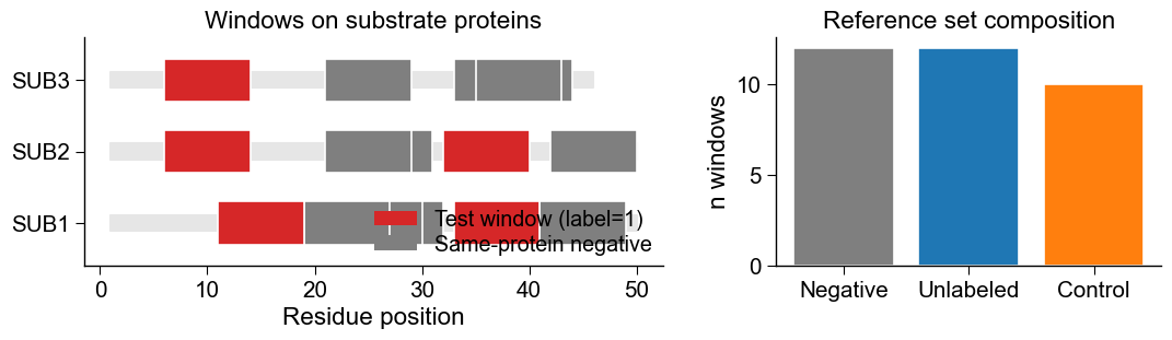
Output. A few things happened across those four calls, so let’s lay the result out and look at it. Notice how the sampled negatives hug the positives along each substrate protein: that is exactly the fair reference this protocol asks for, drawn around the test windows, not from some unrelated corner of the sequence. The panel on the right then tallies the role composition of the assembled reference set.
The sampler returns a segments-mode DataFrame, one row per window,
with the fixed schema
entry_win, entry, sequence, window, source_position, label, role, strategy
(the benchmark set adds arm).
``entry_win``:
"<entry>_<start>-<end>"(1-based inclusive) for protein-sourced windows; identical biological windows across calls share it, sodrop_duplicates(subset="entry_win")is the natural cross-call dedupe.synthetic rows use
entry_win="synth_{i}"(per-call counter), not call-stable; dedupe control windows on thewindowstring instead.
import matplotlib.pyplot as plt
import seaborn as sns

# House style + one consistent colour per role (gray=Negative, blue=Unlabeled, orange=Control, red=Test).
aa.plot_settings(font_scale=0.9, weight_bold=False)
c_neg, c_unl, c_test, c_ctrl = aa.plot_get_clist(n_colors=4)
role_colors = {"Negative": c_neg, "Unlabeled": c_unl, "Control": c_ctrl}

fig, axes = plt.subplots(1, 2, figsize=(11, 3.4), gridspec_kw={"width_ratios": [3, 2]})

# Panel A: where windows sit on the three substrate proteins (a fair reference hugs the positives).
ax = axes[0]
substrates = ["SUB1", "SUB2", "SUB3"]
for i, entry in enumerate(substrates):
    row = df_seq[df_seq["entry"] == entry].iloc[0]
    ax.broken_barh([(1, len(row["sequence"]))], (i - 0.11, 0.22), color="0.9", zorder=1)
    for s in df_same.loc[df_same["entry"] == entry, "source_position"]:   # sampled same-protein negatives
        ax.broken_barh([(s - half_left, 8)], (i - 0.30, 0.60), color=c_neg,
                       edgecolor="white", linewidth=1.2, zorder=2)
    for p in row["pos"]:                                                  # known test windows at P1 anchors
        ax.broken_barh([(p - half_left, 8)], (i - 0.30, 0.60), color=c_test,
                       edgecolor="white", linewidth=1.2, zorder=3)
ax.set_yticks(range(len(substrates)))
ax.set_yticklabels(substrates)
ax.set_ylim(-0.6, len(substrates) - 0.4)
ax.set_xlabel("Residue position")
ax.set_title("Windows on substrate proteins", size=aa.plot_gcfs())
sns.despine(ax=ax)
aa.plot_legend(ax=ax, dict_color={"Test window (label=1)": c_test, "Same-protein negative": c_neg},
               n_cols=1, loc="lower right", fontsize=aa.plot_gcfs() - 2)

# Panel B: role composition of the assembled reference set.
ax = axes[1]
counts = df_bench["role"].value_counts()
ax.bar(counts.index, counts.values,
       color=[role_colors.get(r, "0.5") for r in counts.index],
       edgecolor="white", linewidth=1.2)
ax.set_ylabel("n windows")
ax.set_title("Reference set composition", size=aa.plot_gcfs())
sns.despine(ax=ax)

plt.tight_layout()
# Dedupe correctly per provenance: entry_win for protein-sourced, window for synthetic.
is_synth = df_bench["strategy"].str.startswith("synthetic")
df_protein = df_bench[~is_synth].drop_duplicates(subset="entry_win")
df_control = df_bench[is_synth].drop_duplicates(subset="window")
df_clean = pd.concat([df_protein, df_control], ignore_index=True)
# df_clean is the assembled window set fed to feature engineering (Protocol 4).
aa.display_df(df=df_clean["role"].value_counts().reset_index(), n_rows=3)
| role | count | |
|---|---|---|
| 1 | Negative | 12 |
| 2 | Unlabeled | 12 |
| 3 | Control | 10 |
How to interpret. Read the table one row at a time, each row is a single window, and the columns tell you where it came from and what it means for training:
Column / value |
Reading |
|---|---|
one row |
one fixed-length window anchored at a P1 site |
|
the residue slice the model/CPP actually sees |
|
the 1-based P1 anchor on the
source protein ( |
|
within-protein hard negative (looks local-similar, not a site) |
|
cross-protein site of unknown
status, the |
|
synthetic composition baseline (null) |
|
window-level target ( |
Notice how the set you assemble is the contrast the downstream residue-level CPP run profiles: test vs. all reference, or test vs. a single role (e.g. hard negatives only). Choosing roles is choosing the biological question.
Key takeaways
One row = one fixed-length window; its role (
Test/Negative/Unlabeled/Control) is the workflow meaning you assign, while its strategy is the sampling provenance set for you.Choosing which roles enter the reference group (
label=0) is choosing the biological question: the residue-level CPP contrast is only ever as fair as the reference and control windows you draw.entry_winis the dedupe key for protein-sourced windows across calls; synthetic control windows carry a per-callentry_win, so dedupe them on thewindowstring instead.
Common mistakes.
Feeding pre-windowed data to the sampler:
AA_CASPASE3fromload_dataset()is already windowed; the sampler needs full sequences + a ``pos`` column.Forgetting ``pos_col``: without the P1 anchors the sampler cannot identify positives (to exclude them and to drive the anti-leakage filter).
Wrong ``window_size`` parity: cleavage is between residues (an even window); a single-residue PTM needs an odd window. Match the biology.
Over-sampling a tiny pool: large
nwith few proteins triggers slow re-draws and a shortfall warning; keepn≈ 10× the number of eligible proteins.Mixing roles without intent: decide upfront: PU-learning (
Unlabeled)? hard negatives (Negative)? composition control (Control)?Naive dedupe:
drop_duplicates("entry_win")is right for protein-sourced rows but wrong for synthetic (per-callentry_win); dedupe controls onwindow.
Next step. The clean window set is now the input to P4: Prediction
levels, where the window strings become a df_seq whose
parts are named by the Schechter–Berger convention
(… P2·P1 │ P1′·P2′ …), built with get_df_parts()
and then profiled by run() exactly as in P1: CPP signature (now
at the residue level), or fed as dict_num parts to run_num().