P10: Validation

This protocol is the validation gate: a short, ordered battery of internal sanity checks that asks whether a CPP signature (from P1: CPP signature) and any classifier you build on it can be trusted before you attach a biological claim to a number. A signature can look convincing on a few dozen sequences and still be an artefact of overfitting, leakage, or plain luck, so we validate a determinant-discovery result by asking: would it survive resampling and a shuffled-label control?

Key mental model. A result you cannot reproduce, and cannot beat a shuffled-label control with, is not a result. Validation is not about squeezing out a higher score; it is about proving the score tracks the labels (the real test group vs reference group contrast) and not noise. The single most informative line in this entire protocol is real vs shuffled: if scrambling the labels does not destroy performance, the pipeline is leaking and no other number can be trusted.

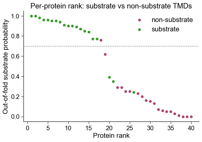
The headline output is a single figure (the per-protein rank plot below, where substrate TMDs rank above non-substrates), backed by the real-vs-shuffled control further down that proves the ranking tracks the labels and not noise.

When to use it. Use this protocol after you have a signature and/or a fitted classifier, and before you report a number or draw a biological conclusion. It answers the reviewer’s first question: “Is this real, or did the model just memorise 40 sequences?”

We stay on the gamma-secretase task (DOM_GSEC), a domain-level problem: the unit of comparison is the transmembrane-domain (TMD) part set, the test group is substrate TMDs (label=1) and the reference group is non-substrate TMDs (label=0). A trustworthy result means the physicochemical separation captured by the signature is stable under resampling and survives the controls below, not that we fit noise.

The checklist mirrors six questions:

Check	Question it answers
Repeated stratified CV	Does performance hold across many train/test splits, not one lucky one?
Bootstrap CI of the mean	How wide is the uncertainty band around the score?
Shuffled-label control	Does the score collapse when the labels carry no information?
Feature stability	Do the top features keep their effect sizes under resampling?
Biological sense	Do the strongest features match known biology?
Generalization headroom (learning curve)	Is the task sampling-limited: would more TMDs still raise the score, or has it plateaued?

When not to use it. All six checks are internal: they resample the same 40 TMDs and cross-validate in-sample. They tell you whether a result is stable and not an artefact; they do not measure external generalization. If your question is “will this signature transfer to a different dataset?”, this protocol is not enough: you need a true external hold-out (a separate, unseen set of proteins). And do not reach for this protocol before you have a signature: build one first with P1: CPP signature.

Input. The same input as P1: CPP signature: a df_seq with one row per protein, a binary label column (test group = 1, reference group = 0) and the domain coordinates (tmd_start / tmd_stop). We rebuild the signature (df_feat) and the feature matrix X exactly as in P1, then validate them.

If you arrived here straight from P1 you already have df_feat and X; the cell below reproduces them so this protocol stands on its own. We keep the fixture small (n=20, giving 40 balanced TMDs) and the cross-validation light, so the whole checklist runs in seconds.

import warnings
import numpy as np
import aaanalysis as aa

aa.options["verbose"] = False
aa.options["random_state"] = 42

# Rebuild the Protocol 1 signature on a small balanced fixture
df_seq = aa.load_dataset(name="DOM_GSEC", n=20)      # 20 per class -> 40 rows
labels = np.array(df_seq["label"].to_list())

sf = aa.SequenceFeature()
df_parts = sf.get_df_parts(df_seq=df_seq)
cpp = aa.CPP(df_parts=df_parts)
df_feat = cpp.run(labels=labels, n_filter=25, n_jobs=1)

# Feature matrix: rows = TMDs, columns = the 25 selected features
X = sf.feature_matrix(features=df_feat["feature"], df_parts=df_parts)
X.shape, df_feat.shape

((40, 25), (25, 13))

Run. Each check is one small cell. We use a RandomForestClassifier as a neutral downstream model and the Matthews correlation coefficient (MCC) as the headline metric: MCC is balanced, ranges from -1 to 1, and reads ~0 for a model that has learned nothing, which is exactly what makes the shuffled-label control easy to read. (AAanalysis ships its own tree classifier, aa.TreeModel, whose .eval scores feature-set quality with k-fold CV (see the comparison-harness tutorial, tutorial6, for the function details); for the native-evaluator path see P7: Build a classifier. Here we drive a raw RandomForest so every control stays explicit and framework-agnostic.)

Check 1: repeated stratified cross-validation. RepeatedStratifiedKFold keeps the 50/50 class balance in every fold and repeats the whole split several times, so the score is an average over many train/test partitions rather than one lucky one.

from sklearn.ensemble import RandomForestClassifier
from sklearn.model_selection import RepeatedStratifiedKFold, cross_val_score
from sklearn.metrics import matthews_corrcoef, make_scorer

clf = RandomForestClassifier(n_estimators=100, random_state=42)
cv = RepeatedStratifiedKFold(n_splits=5, n_repeats=3, random_state=42)  # 15 fits
mcc = make_scorer(matthews_corrcoef)

scores = cross_val_score(clf, X, labels, cv=cv, scoring=mcc)
float(scores.mean()), float(scores.std())

(0.8070022769184196, 0.17911074334561763)

Headline figure: per-protein rank plot. The deployment-view sanity check. We turn the cross-validation into one out-of-fold substrate probability per TMD (every protein scored only by folds that never saw it), then rank proteins high-to-low with aa.plot_rank and color each by its true group. A trustworthy signature ranks substrate TMDs (test group) above non-substrate TMDs (reference group); the dashed line is the deployment threshold a caller would apply. This is the single most useful one-glance check, and the controls below (starting with real vs shuffled) are what make the separation believable.

# Headline figure: per-protein rank plot (the deployment-view sanity check)
# One out-of-fold substrate probability per TMD: each protein is scored only by
# the folds that never trained on it, so the ranking is honest (no leakage).
import pandas as pd
import matplotlib.pyplot as plt
from sklearn.model_selection import StratifiedKFold, cross_val_predict

cv_pred = StratifiedKFold(n_splits=5, shuffle=True, random_state=42)
proba = cross_val_predict(clf, X, labels, cv=cv_pred, method="predict_proba")[:, 1]
df_rank = pd.DataFrame({
    "score": proba,
    "group": np.where(labels == 1, "substrate", "non-substrate"),
})

aa.plot_settings(font_scale=0.9, weight_bold=False)
fig, ax = aa.plot_rank(df_rank=df_rank, threshold=0.7,
                       ylabel="Out-of-fold substrate probability")
ax.set_title("Per-protein rank: substrate vs non-substrate TMDs",
             size=aa.plot_gcfs() + 1)
plt.tight_layout()
plt.show()

../_images/protocol10_validation_1_output_7_0.png

Check 2: bootstrap confidence interval. comp_bootstrap_ci resamples the 15 fold scores with replacement (seed-locked) to put a 95% interval around the mean MCC, so we report a band rather than a bare point estimate.

# Check 2 - Bootstrap confidence interval of the mean MCC
# comp_bootstrap_ci resamples the 15 fold scores with replacement (seed-locked).
ci = aa.comp_bootstrap_ci(values=scores, n_rounds=1000, ci=0.95, seed=42)
ci

{'mean': 0.8070022769184196,
 'ci_low': 0.7139891620269944,
 'ci_high': 0.8967358359109805}

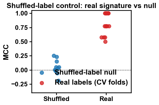
Check 3: shuffled-label (negative) control. The single most informative check, and the one the Key mental model rests on: permute the labels so they carry no information and confirm the score collapses toward MCC ~ 0. We average over several reshuffles so the null is a mean over many draws, not one noisy point. The figure just below makes the gap visible. Here we average over only 10 permutations to stay inside the per-cell time budget; a production run should use many more (e.g. >=100) for a smoother null.

# Check 3 - Shuffled-label (negative) control
# Permute the labels many times: any structure left is pure chance. A
# trustworthy signature collapses toward MCC ~ 0 here. We average over
# several reshuffles so the null is a mean over many splits, not a single
# noisy point estimate (the same 'many resamples' logic as Check 1).
rng = np.random.default_rng(42)
shuffled_means = []
with warnings.catch_warnings():
    warnings.simplefilter("ignore")          # degenerate shuffled folds -> expected MCC warnings
    for _ in range(10):
        labels_shuffled = rng.permutation(labels)
        s = cross_val_score(clf, X, labels_shuffled, cv=cv, scoring=mcc)
        shuffled_means.append(s.mean())
{"real_MCC": round(float(scores.mean()), 3),
 "shuffled_MCC_mean": round(float(np.mean(shuffled_means)), 3),
 "shuffled_MCC_max": round(float(np.max(shuffled_means)), 3)}

{'real_MCC': 0.807, 'shuffled_MCC_mean': 0.051, 'shuffled_MCC_max': 0.252}

A few things happened here. The figure contrasts the 15 real cross-validation fold scores (right) against the shuffled-label null (left). This is the protocol’s key control picture, the one that backs the rank plot above: notice how the two clouds barely overlap, the real folds sit high while the shuffled control hugs MCC ~ 0. That obvious gap is the evidence that the signature tracks the labels, not chance.

# Headline figure: shuffled-label control (the Key mental model, made visible)
import matplotlib.pyplot as plt
aa.plot_settings()
c_null, c_real = aa.plot_get_clist(n_colors=2)  # consistent with the CPP figures

fig, ax = plt.subplots(figsize=(5, 4))
jit = np.random.default_rng(0)
x_shuf = jit.normal(0.0, 0.04, size=len(shuffled_means))
x_real = 1 + jit.normal(0.0, 0.04, size=len(scores))
ax.scatter(x_shuf, shuffled_means, color=c_null, alpha=0.8, label="Shuffled-label null")
ax.scatter(x_real, scores, color=c_real, alpha=0.8, label="Real labels (CV folds)")
ax.axhline(0, color="black", lw=0.8, ls="--")
ax.set_xticks([0, 1])
ax.set_xticklabels(["Shuffled", "Real"])
ax.set_xlim(-0.5, 1.5)
ax.set_ylim(-0.4, 1.05)
ax.set_ylabel("MCC")
ax.set_title("Shuffled-label control: real signature vs null")
ax.legend(frameon=False, loc="lower center")
plt.tight_layout()
plt.show()

../_images/protocol10_validation_2_output_13_0.png

Check 4: feature stability under resampling. Recompute each feature’s adjusted-AUC effect size on bootstrap resamples and correlate it with the full-data effect sizes. A high correlation means the signature reflects real effect sizes, not resampling noise. We use just 5 bootstrap resamples here for speed; on a real study raise this to >=100 so the stability estimate is not itself noisy.

# Check 4 - Feature stability under resampling
# Recompute the adjusted AUC (effect size, [-0.5, 0.5]) for every feature on
# bootstrap resamples and correlate it with the full-data effect sizes.
# High correlation = the signature's effect sizes are not resampling artefacts.
# Re-seed here so this cell is reproducible on its own (not dependent on the
# RNG state left by Check 3).
rng = np.random.default_rng(42)
auc_full = aa.comp_auc_adjusted(X=X, labels=labels)
corrs = []
for _ in range(5):
    idx = rng.choice(len(labels), size=len(labels), replace=True)
    while len(np.unique(labels[idx])) < 2:          # keep both classes present
        idx = rng.choice(len(labels), size=len(labels), replace=True)
    auc_b = aa.comp_auc_adjusted(X=X[idx], labels=labels[idx])
    corrs.append(np.corrcoef(auc_full, auc_b)[0, 1])
round(float(np.mean(corrs)), 3)

0.992

Check 5 and 6: biological sense and generalization headroom (learning curve). Read the strongest features against known substrate biology, then use a learning curve to ask whether the task is sampling-limited: would more TMDs still raise the score, or has the signal plateaued?

For DOM_GSEC, the expected substrate physicochemistry around the cleavage site is helix-destabilizing / helix-breaking propensity, β-turn and flexibility signals (a locally less rigid, more bendable helix lets gamma-secretase unwind and cleave the TMD). So α-helix, β-turn and folding free-energy subcategories topping the list is the biologically sensible outcome; charge or bulky-hydrophobicity terms dominating instead would be a red flag.

Note: this is internal in-sample cross-validation over the same 40 TMDs, it measures sampling headroom, not external generalization. A true external-generalization estimate needs a separate hold-out dataset.

# Check 5/6 - Biological sense + generalization headroom (learning curve)
# Top features by effect size: do the strongest physicochemical properties
# match known substrate biology? For DOM_GSEC we expect helix-destabilizing /
# β-turn / flexibility signals near the cleavage site (read the subcategory).
top = df_feat.reindex(df_feat["abs_auc"].sort_values(ascending=False).index)
aa.display_df(df=top[["feature", "category", "subcategory", "mean_dif", "abs_auc"]], n_rows=5)

# Learning curve (INTERNAL in-sample CV, no external hold-out): does the score
# still climb with more TMDs (the task is sampling-limited, more data would
# help) or has it plateaued (the signal is captured)? We start at 0.6 of the
# training fold so the smallest size keeps both classes (a smaller size makes
# MCC undefined, the tiny-fold trap flagged under Common mistakes).
from sklearn.model_selection import learning_curve
with warnings.catch_warnings():
    warnings.simplefilter("ignore")
    sizes, train_sc, test_sc = learning_curve(
        clf, X, labels, cv=cv, scoring=mcc,
        train_sizes=np.linspace(0.6, 1.0, 4))
{"train_sizes": sizes.tolist(),
 "test_MCC_by_size": np.round(test_sc.mean(axis=1), 3).tolist()}

	feature	category	subcategory	mean_dif	abs_auc
1	TMD-Pattern(C,4,8)-BEGF750101	Conformation	α-helix	0.299000	0.444000
2	TMD_C_JMD_C-Pat...4,8)-BEGF750101	Conformation	α-helix	0.299000	0.444000
3	TMD_C_JMD_C-Pat...,12)-CRAJ730103	Conformation	β-turn	-0.251000	0.431000
4	TMD_C_JMD_C-Pat...,12)-MUNV940102	Energy	Free energy (folding)	-0.148000	0.422000
5	TMD_C_JMD_C-Per...4,2)-BEGF750103	Conformation	β-turn	-0.139000	0.409000

{'train_sizes': [19, 23, 27, 32],
 'test_MCC_by_size': [0.696, 0.778, 0.792, 0.807]}

Output. The headline output is the per-protein rank plot above: substrate TMDs ranking above non-substrates, with the deployment threshold drawn in. Its credibility rests on the real-vs-shuffled figure, where the wide vertical gap between the real cross-validation fold scores and the shuffled-label null is the evidence that the ranking tracks the labels. Everything else is a small panel of scalars you can paste straight into a methods section:

df_rank: one out-of-fold substrate probability per TMD plus its true group, the table behind the rank plot.
scores.mean() / scores.std(): mean repeated-CV MCC and its spread across 15 fits.
ci: dictionary {'mean', 'ci_low', 'ci_high'}, the 95% bootstrap interval of the mean MCC. Caveat: the 15 RepeatedStratifiedKFold folds share most of their training data, so they are not independent samples; bootstrapping them understates uncertainty, making this band a lower bound on the true interval. The only honest test of generalization is an external hold-out.
real_MCC vs shuffled_MCC_mean / shuffled_MCC_max: the headline score against its negative control, averaged (and worst-cased) over 10 independent label permutations.
the stability correlation: mean Pearson correlation of per-feature effect sizes across bootstrap resamples (1.0 = an identical effect-size profile every time).
top: the five strongest features for the biological-sense eyeball check.
test_MCC_by_size: MCC as a function of training-set size (the learning curve).

How to interpret. Each output maps to a trustworthy reading and a warning sign:

Output	Trustworthy result	Warning sign
repeated-CV `MCC`	high and stable (low `std`)	high mean but large `std` -> split-dependent
bootstrap `ci`	narrow, well above 0	wide band crossing ~0 -> under-powered
`shuffled_MCC_mean`	collapses far below the real MCC (toward 0)	stays high -> leakage / the metric is not measuring signal
stability correlation	close to 1.0	low / variable -> effect sizes are resampling noise
`top` features	subcategories match expected GSEC-substrate biology (helix-destabilizing / β-turn / flexibility near the cleavage site)	top features biologically implausible (e.g. charge / bulk dominating) -> suspect overfitting
learning curve (internal CV)	rising then plateauing	flat and low -> features carry little signal; still steeply rising -> task is sampling-limited, more data needed

On this fixture the real MCC sits high while the shuffled control drops sharply toward 0: the separation tracks the labels, not an artefact.

Key takeaways

Real vs shuffled is the gate. If scrambling the labels does not destroy performance, the pipeline is leaking and every other number is meaningless. Always run the negative control first.
Report a band, never a point. With only 40 TMDs every number is under-powered; quote the bootstrap interval, not a bare MCC.
Internal is not external. All six checks resample the same TMDs. Surviving them earns trust in stability, not a promise of transfer: confirm external generalization on a separate dataset.

Common mistakes. The traps below sink most validation attempts:

No shuffled-label control. A high CV score alone proves nothing; only the gap between real and shuffled performance does. Always run the negative control.
Plain K-fold instead of stratified. With 40 rows an unstratified split can leave a fold with one class, making MCC undefined or wildly unstable. Use RepeatedStratifiedKFold.
Reporting a point estimate. A single MCC hides the uncertainty. Report the bootstrap CI (comp_bootstrap_ci) of the mean.
Re-selecting features inside the loop is skipped here for speed. On a real study, run CPP feature selection inside each CV fold to avoid selection leakage; reusing one global df_feat mildly optimistically biases the score.
Over-reading a single feature. Interpret the signature as blocks of related features; check effect-size stability before any biological claim.
Using ``len(df_seq)`` for class sizes. load_dataset(name=..., n=N) returns 2N rows (N per class); use the label column.

Next step. You have run the internal validation gate: repeated stratified CV with a bootstrap CI, a shuffled-label control, feature-stability under resampling, a biological-sense read and a learning curve. If the result survived all of them it is ready to report, with the standing caveat that external generalization still needs a separate hold-out dataset.

Loop back to P1: CPP signature and apply the whole workflow to a new dataset: the surest external-generalization test is to rebuild the signature on a fresh, unseen set of proteins and re-run this validation gate there.
Revisit P1: CPP signature sooner if a control failed: rebuild or tighten the signature before you report a number.
Quantify uncertainty per protein for residue-level / windowed site-prediction tasks (not this domain task), pairing comp_per_protein_ap with comp_bootstrap_ci for protein-level confidence intervals.